The A-Z guide to Support Vector Machine
This article was published as a part of the Data Science Blogathon
Introduction
Support Vector Machine (SVM) is one of the Machine Learning (ML) Supervised algorithms. There are plenty of algorithms in ML, but still, reception for SVM is always special because of its robustness while dealing with the data. So here in this article, we will be covering almost all the necessary things that need to drive for any kind of data w.r.t SVM. Before getting deep into the topic, let us get wet by brushing up on some of the basic terminology related to SVM. I hope you will enjoy it! It might be a bit lengthy and sure it won’t disappoint you!
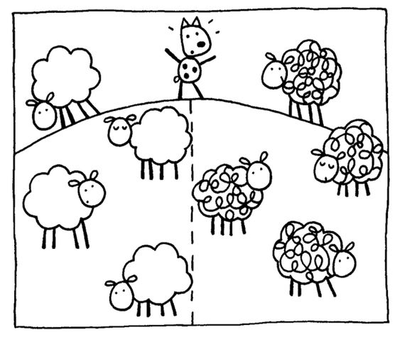
Table of contents
- Introduction
- Machine Learning – Teaser Introduction (Basic Intro):
- SVM – Maximal Margin Classifier – First Song:
- Support Vector Classifier (SVC)(Second Song):
- Support Vector Machine (SVM) – (Interval block):
- Basic Parameters for SVM – (Dramatic/Side portion) (both linear and non-linear SVMs)
- Random State:
- Coding Part (Behind the Scenes!)
- End Notes:
Machine Learning – Teaser Introduction (Basic Intro):
Machine Learning algorithm (set of rules to achieve some outcome), means it can access the data (categorical, numerical, image, video, or anything) and use it to learn for themselves without any programming (like without order means or sequential steps to do!). But still how it works? by simply observing the data (through instructions to observe the pattern and making decision or prediction)
Machine Learning is the field of study that gives computers the ability to learn without being explicitly programmed. —Arthur Samuel, 1959
ML is classified into three broad main domains,
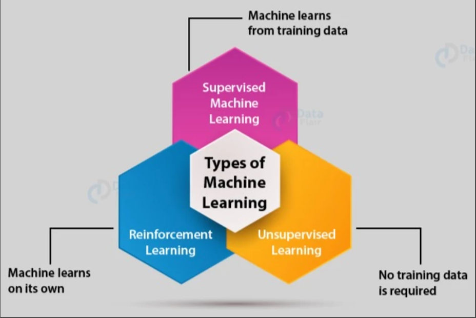
In simple terms,
1. Supervised ML – Dataset/data has features (independent variables) and target (dependent variable/target) variables. It has two broad types: Classification and Regression.
2. Unsupervised ML – Dataset/data having features alone or without target variables. Again classified into Clustering, Anomaly Detection, Dimensionality reduction, Association rule-based learning.
3. Reinforcement ML – This domain is something different the above two, here simple but complicated rule is learn by rewards and punishments (learning like kids in school)
4. Semi-Supervised Learning (Partial data’s with and without label)
From the above content, it can be concluded that we are dealing with Supervised ML alone in this article. And in reality, the SVM algorithm comes under Supervised ML, and to the surprise, it deals with both Classification and Regression.
So, What is the term Classification and Regression?
1. Classification: Finding a mapping function of the independent variable to identify discrete dependent variable, it can be labels or categories oriented. Here, the dependent variable is a qualitative type like binary or multi-label types like yes or no, normal or abnormal, and categorical types like good, better, best, type 1 or type 2, or type 3. Ex: Finding our mail between spam or not.
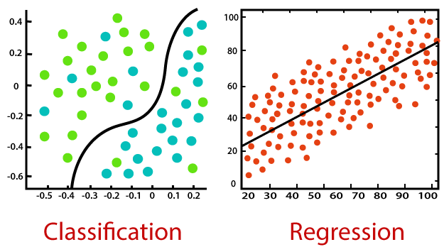
2. Regression: Finding a correlation (mapping function) between the independent variable and dependent variable. Another important function is to predict a continuous value based on the independent variables. Here there won’t be any classes like in classification, instead of classes, if the dependent variable is in quantity like height, weight, income, rainfall prediction, or share market prediction, we go for the regression technique. Ex: Predicting rain for the next 5 days.
SVM is a special algorithm, which is represented in classification and regression.
Support Vector Machine – Fan-Made Poster release (MEME Introduction):
I always believe, “A picture is worth a thousand words“, so before we get into the SVM ocean, we will understand the whole concept in the below picture, it suits the current situation (COVID-19) too,

SVM – Hero Introduction (Theoretical Introduction):
1. SVM – Comes under Supervised ML
2. SVM can perform both Classification & Regression
3. Goal – Create the best decision boundary that can segregate n-dimensional space into classes so that we can easily put the new data points in the correct category – Hyperplane.
4. Out-of-the-box classifier
5. For a better understanding of SVM, we will learn,
@ Maximal Margin Classifier
@ Support Vector Classifier
@ Support Vector Machine
SVM – Maximal Margin Classifier – First Song:
Before we know about Maximal Margin Classifier (MMC), let us start from the basics, we all know the terms 1 Dimensional (1D), 2 Dimensional (2D), and 3 Dimensional (3D). So what it is?
In short, Dimension means measurement (total amount of measurable space or surface occupied). In simple, a number of dimensions are how many values are needed to locate points on a shape.
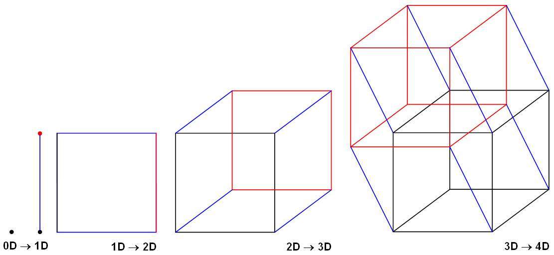
1. No dimension or 0-D – A point (the only position exists)
A point really has no size at all! But we show them as dots so we can see where they are!
2. One dimension or 1-D – A-line (with two points)
Now let’s allow the point to move in one direction. We get a line. We need just one value to find a point on that line.
3. Two-dimension or 2-D – A-plane
Now let us allow the point to move in a different direction. And we get a plane. We need two values to find a point on that plane.
4. Three dimensions or 3-D – A-Solid (maybe a cube)
Now we let that point move in another completely different direction and we have three dimensions.
Note: A point is a hyperplane in 1-dimensional space, a line is a hyperplane in 2-dimensional space, and a plane is a hyperplane in 3-dimensional space.
So now I hope we get some clarity w.r.t the dimensionality concept. So here for SVM, we will be using a term called HYPERPLANE, this plays important role in classifying the data into different groups (will see in detail very soon here in this article!).
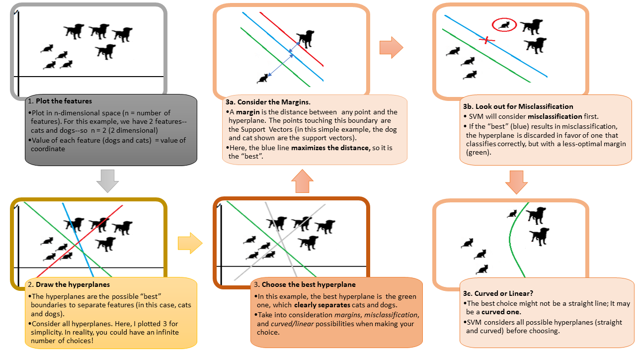
Let us assume from the below-given figure, we have a dataset that has X1 and X2 as independent features and Category as a dependent feature, sometimes we call it as target or label,
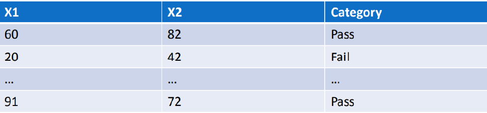
Let us assume, from the above-mentioned dataset with 2 independent features (X1 & X2) are plotted in 2D space or graph in simple and separated by a line for class category (Pass or Fail).
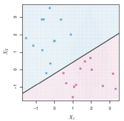
There are many possibilities to separate the two category classes – But which is best among all?
We cannot predict it right, so the solution for the problem is HYPERPLANE. It can be picturized by the below figure in a generalized way,
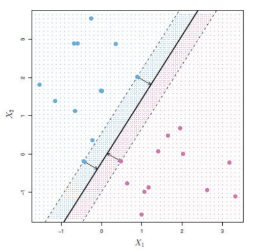
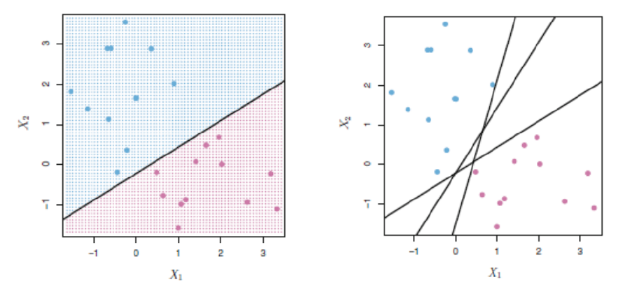
So, among these different hyperplanes, which is the best hyperplane?
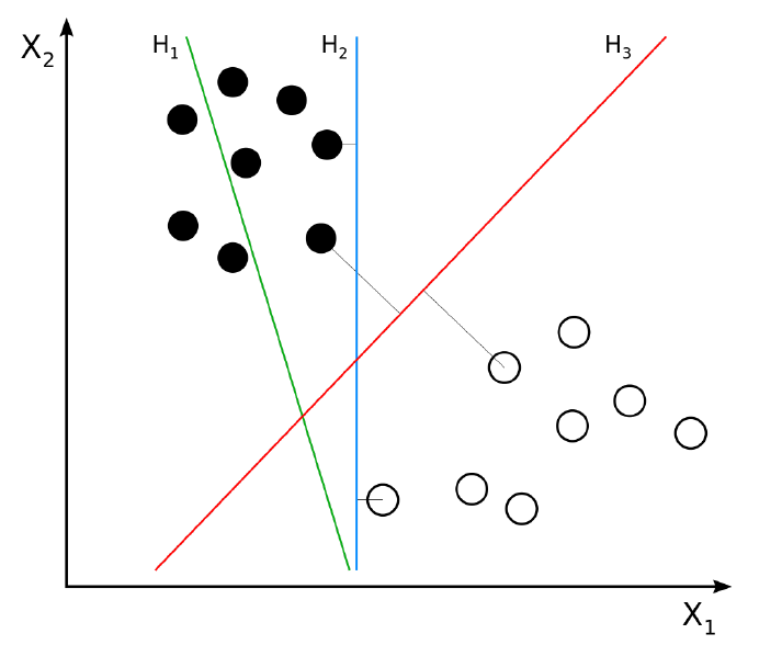
If you observed in the above figure, we can clearly see like among three-line, red line (H3) which has the maximum margin with the data points and also classified between the data properly, if you see blue color line (H2) the margin is small with one data and large with another data, whereas, green line (H1), it has not classified between the data itself.
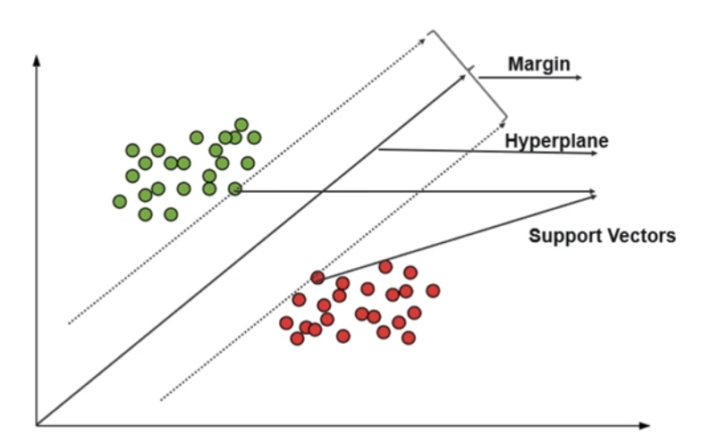
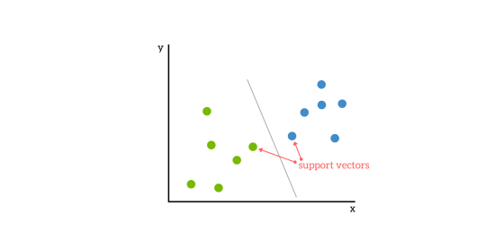
For MMC – Support Vector, Hyperplane, and Margin (Romance Song!)
1. The data/vector points closest to the hyperplane (black line) are known as the support vector (SV) data points because only these two points are contributing to the result of the algorithm (SVM), other points are not.
2. If a data point is not an SV, removing it has no effect on the model.
3. Deleting the SV will then change the position of the hyperplane.
The dimension of the hyperplane depends upon the number of features. If the number of input features is 2, then the hyperplane is just a line. If the number of input features is 3, then the hyperplane becomes a two-dimensional plane. It becomes difficult to imagine when the number of features exceeds 3.
Support Vector Classifier (SVC)(Second Song):
Many have confusion with the terms SVM and SVC, the simple answer is if the hyperplane that we are using for classification is in linear condition, then the condition is SVC.
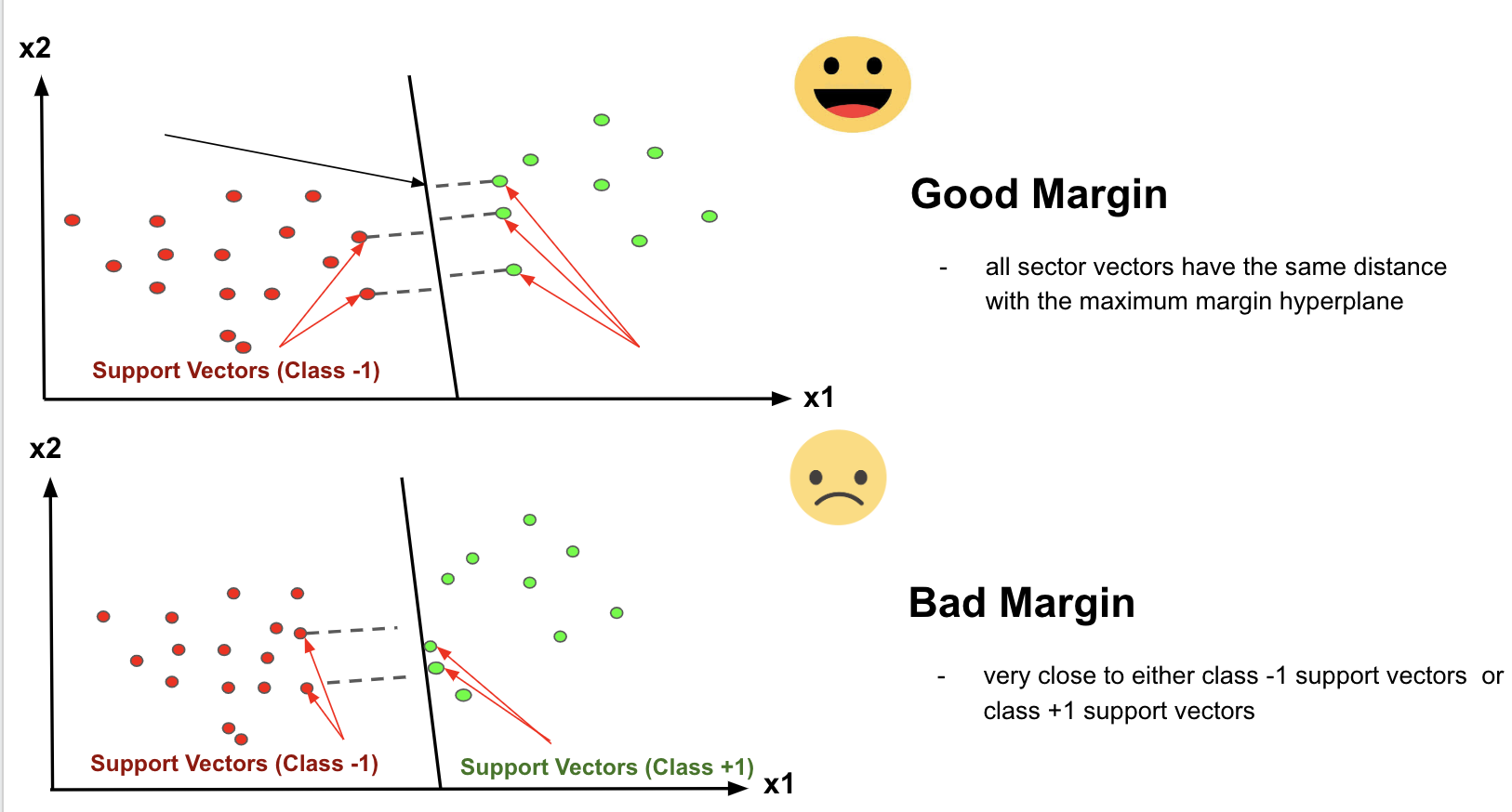
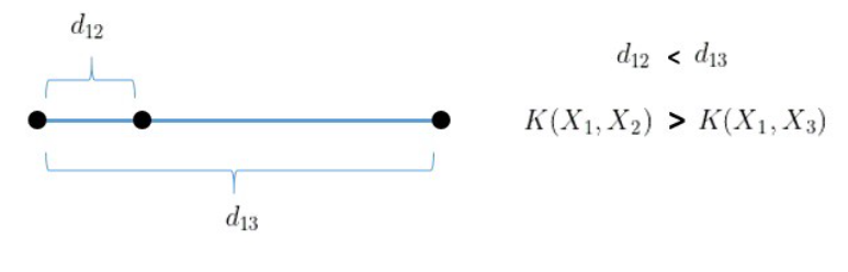
The distance of the vectors from the hyperplane is called the margin which is a separation of a line to the closest class points. We would like to choose a hyperplane that maximizes the margin between classes. The graph below shows what good margins and bad margins are.
Again Margin can be sub-divided into,
1. Soft Margin – As most of the real-world data are not fully linearly separable, we will allow some margin violation to occur which is called soft margin classification. It is better to have a large margin, even though some constraints are violated. Margin violation means choosing a hyperplane, which can allow some data points to stay on either the incorrect side of the hyperplane and between the margin and correct side of the hyperplane.
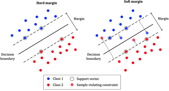
2. Hard Margin – If the training data is linearly separable, we can select two parallel hyperplanes that separate the two classes of data, so that the distance between them is as large as possible.
Note: In order to find the maximal margin, we need to maximize the margin between the data points and the hyperplane.
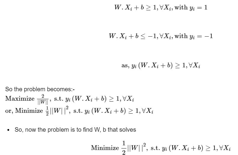
Slight Mathematics (Confused scene):
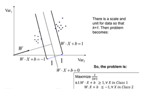
The whole mathematics related with SVM is summarized in both the picture in short, above and below picture,
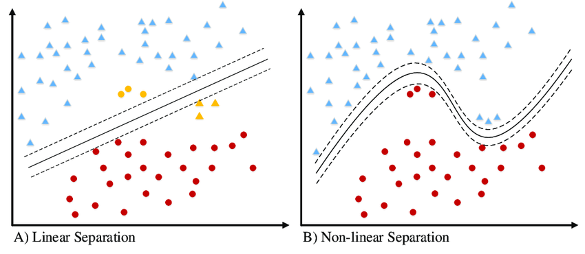
Limitation of SVC (Sudden Twist in the movie):
There are some limitations with SVC, that can be explained by the below picture,
Here in the above picture if you noticed clearly, we cannot draw a hyperplane in this scattered data to separate the data points between classes (for classification!) by a straight line or technically we call it linearly.
Support Vector Machine (SVM) – (Interval block):
The limitation of SVC is compensated by SVM non-linearly. And that’s the difference between SVM and SVC. If the hyperplane classifies the dataset linearly then the algorithm we call it as SVC and the algorithm that separates the dataset by non-linear approach then we call it as SVM.
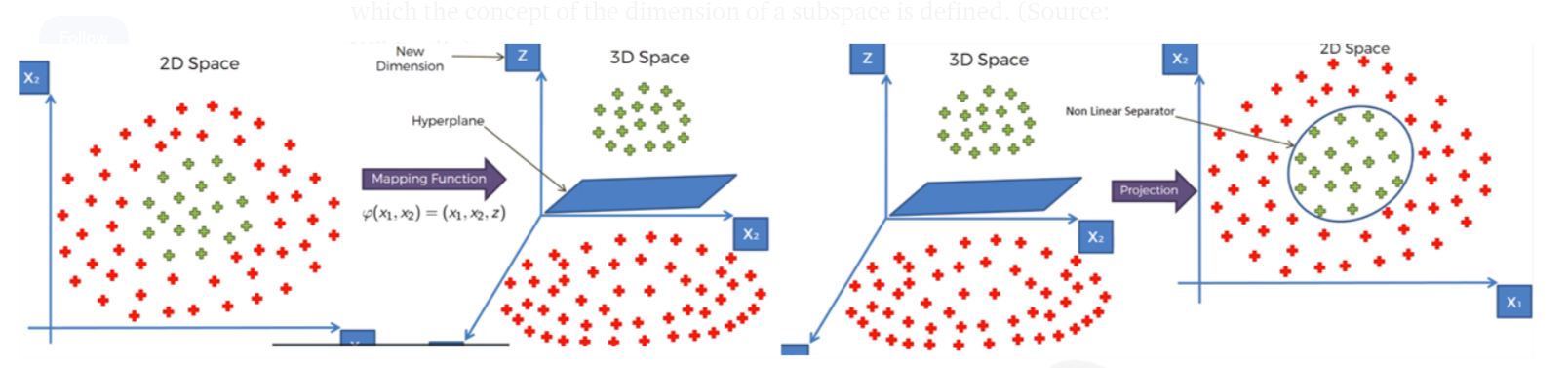
SVM has a technique called the kernel trick. These are functions that take low dimensional input space and transform it into a higher-dimensional space i.e. it converts not separable problem to separable problem.
It is mostly useful in non-linear separation problems. This is shown as follows:
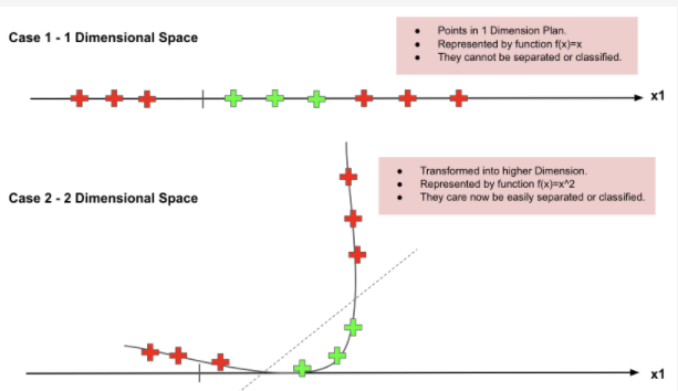
In a more precise manner, Nonlinear can be explained by another visual representation as below, where it can be clearly seen that how the data points which is not able to linearly classified is converted into higher dimensional, then get separated linearly in higher space, which is back non-linearly separated in the original dimension of lower space.
Still confused with the above figures, if you still need more clarity, see the below video for crystal clear idea, how the data are transformed into higher dimensional and from there how linearly got separated then back to the normal plane,
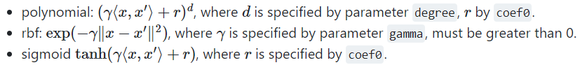
There are some famous and most frequently used Non-linear kernels in SVM are,
1. Polynomial SVM Kernel
2. Gaussian Radial Basis Function (RBF)
3. Sigmoid Kernel
Polynomial SVM Kernel: (#1 Fight Scene!)
1. One way to create features in higher dimensions is by doing polynomial combinations to a certain degree.
2. For instance, with two features A and B, a polynomial of degree 2 would produce 6 features: 1 (any feature to power 0), A, B, A², B², and AB.
3. We can easily add these features manually with scikit-learn’s PolynomialFeatures().
4. The advantage of using this kernelized version is that you can specify the degree to be large, thus increasing the chance that data will become linearly separable in high-dimensional space, without slowing the model down.
Radial Basis Function Kernel: (#2 Fight Scene!)
1. RBF kernels are the most generalized form of kernelization and are one of the most widely used kernels due to their similarity (how close they are to each other) to the Gaussian distribution. Mathematically, RBF
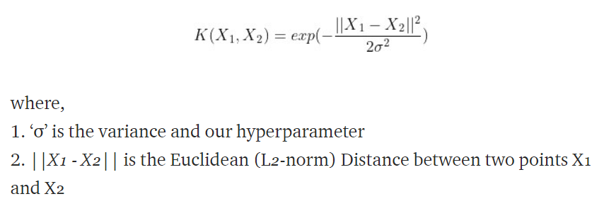
2. Maximum value of RBF kernel is 1 when X1 = X2, which means the distance between the two points X1 and X2 is 0 (Which means it’s extremely similar), If the two points are separated by a large distance (meaning – not similar), then the value will be less than 1 or close to 0.
3. Suppose consider, σ = 1, then it can be explained by,
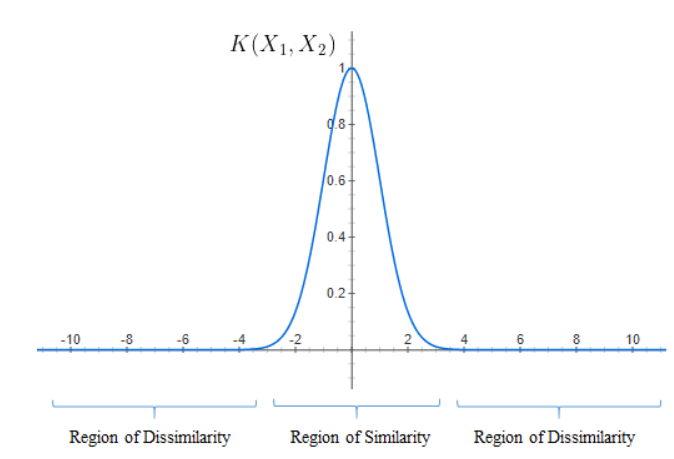
The curve for the RBF equation is shown above and we can notice that as the distance increases, the RBF Kernel decreases exponentially and is 0 for distances greater than 4.
4. Suppose consider, σ = 10, then it can be explained by,
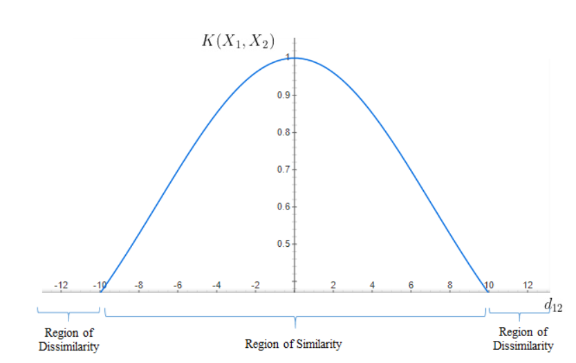
Image Source: image.google.com
The points are considered similar for distances up to 10 units and beyond 10 units are dissimilar. It is evident from both cases that the width of the Region of similarity changes as σ changes.
3. Sigmoid function kernel(#3 Fight Scene!)
1. The Sigmoid Kernel comes from the Neural Networks field, where the bipolar sigmoid function is often used as an activation function for artificial neurons.
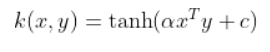
2. It is interesting to note that an SVM model using a Sigmoid kernel function is equivalent to a two-layer, perceptron neural network 3. There are two adjustable parameters in this kernel, Slope – alpha and constant C – intercept.
Basic Parameters for SVM – (Dramatic/Side portion) (both linear and non-linear SVMs)
In scikit-learn (one of the most famous libraries used for Machine Learning algorithms and also for pre-processing steps) for modeling linear and non-linear algorithms, we have plenty of parameters present in the library like as shown below,

We thought we have plenty of parameters option, we will be using only very few alone because of its importance and for its impact,
1. Regularization parameter (C)
2. Gamma parameter
3. Kernel
4. Degree
5. Random state
Regularization parameter (C):
1. The C parameter in SVM is mainly used for the Penalty parameter of the error term.
2. You can consider it as the degree of correct classification that the algorithm has to meet or the degree of optimization the SVM has to meet.
3. Controls the tradeoff between the classification of training points accurately and a smooth decision boundary or in a simple word, it suggests the model choose data points as a support vector.
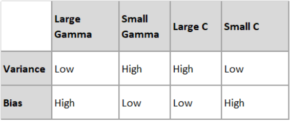
3. For large C – then model choose more data points as a support vector and we get the higher variance and lower bias, which may lead to the problem of overfitting.
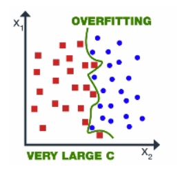
Image Source: image.google.com
4. For small C – If the value of C is small then the model chooses fewer data points as a support vector and gets lower variance/high bias.
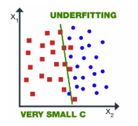
Image Source: image.google.com
The value of gamma and C should not be very high because it leads to overfitting or it shouldn’t be very small (underfitting). Thus we need to choose the optimal value of C.
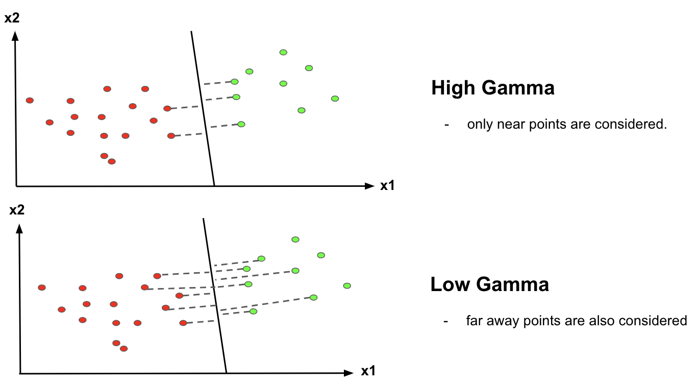
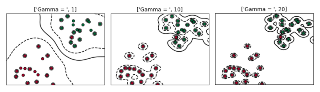
Gamma Parameter:
1. Gamma is used when we use the Gaussian RBF kernel.
2.If you use linear or polynomial kernel then you do not need gamma only you need C hypermeter.
3. It decides that how much curvature we want in a decision boundary.
4. High Gamma value – More curvature
5. Low Gamma value – Less curvature
Hence we need to choose the value of C and gamma wisely for better classification,
********************************************************************************************
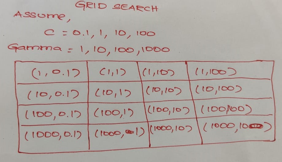
Note: The goal is to find the balance between “not too strict” and “not too loose”. Cross-validation and resampling, along with grid search, are good ways to finding the best C. Then choosing gamma values are associated with C for better accuracy.
********************************************************************************************
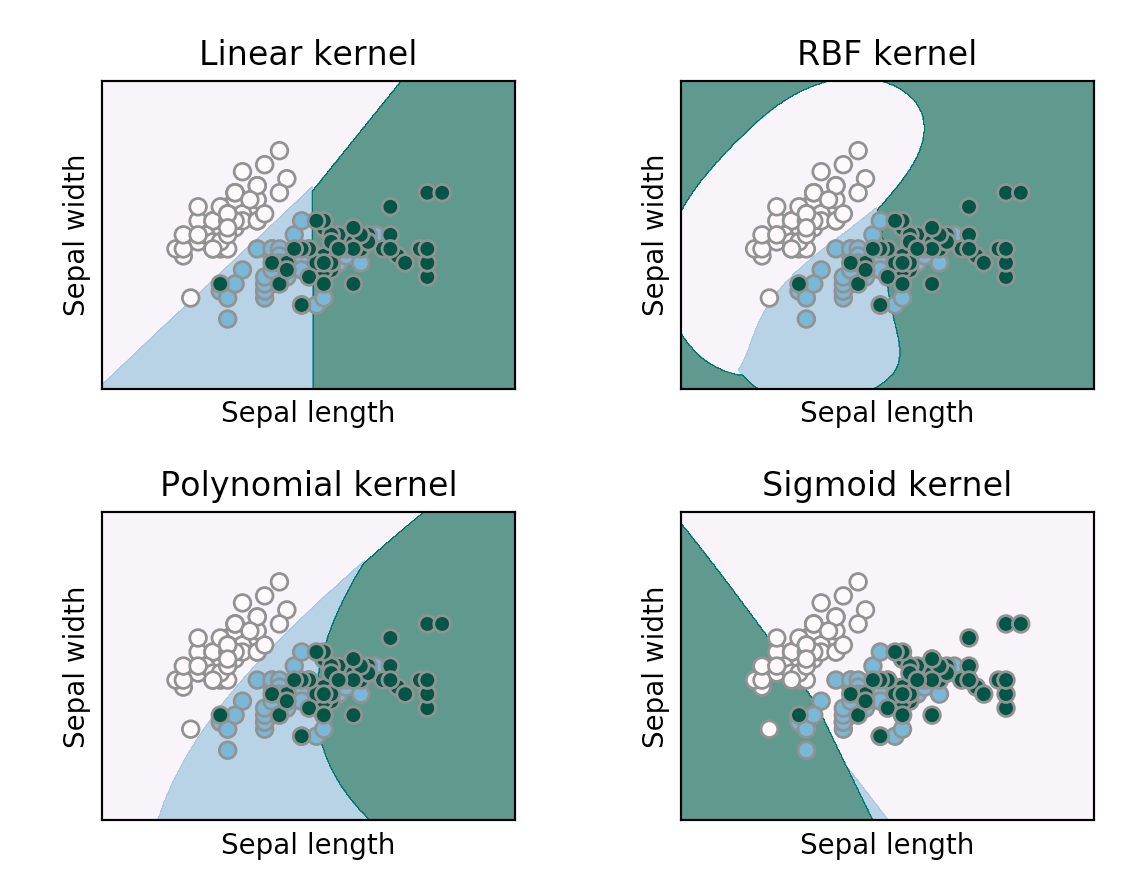
Kernel:
In this parameter, it’s very simple, in this parameter few option’s are there like if you want to model it in a linear manner, we go for ‘linear’ or if your model did not have proper accuracy then you go for non-linear SVM like ‘rbf’, ‘poly’ and ‘sigmoid’ for better accuracy. Let’s assume as like below,
Degree:
1. It controls the flexibility of the decision boundary.
2. Higher degrees yield more flexible decision boundaries.
3. Highly recommended for polynomial kernel
Random State:
This particular parameter, 50-50 people use it and others won’t. This is not so important, ensures that the splits that you generate are reproducible, like we give mostly the value as 0 or 1 or it may be any other number too.
SVM – Summary (Towards Climax Scene):
SVM – Advantage, Disadvantage & Applications (Climax Scene):
Advantage:
1. More effective for high dimensional space
2. Works well with even unstructured and semi-structured data like text, Images, and trees
3. Handles non-linear data efficiently by using the kernel trick
4. SVM has an L2 Regularization feature. So, it has good generalization capabilities which prevent it from over-fitting
5. A small change to the data does not greatly affect the hyperplane and hence the SVM. So the SVM model is stable
Disadvantage:
1. Not suitable for large dataset
2. Sensitive to outliers (If you have more in the dataset then SVM is not the right choice!)
3. Hyperparameters like cost (C) and gamma of SVM, is not that easy to fine-tune and also hard to visualize their impact
4. SVM takes a long training time on large datasets
5. SVM model is difficult to understand and interpret by human beings, unlike Decision Trees.
6. One must do feature scaling of variables before applying SVM
Applications:
1. Handwriting recognition
2. Face Detection
3. Text and hypertext categorization
4. Image Classification
5. Bioinformatics (protein classification and cancer classification)
SVM Cheat Sheet (Movie End Credit):
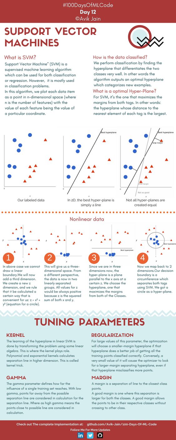
Image Source: github.com
Coding Part (Behind the Scenes!)
Dataset & Full Code: https://github.com/anandprems/SVM_Classification_Regression
SVM – Classification:
import numpy as np
import pandas as pd
import matplotlib.pyplot as plt
import seaborn as sns
%matplotlib inline
dataset = pd.read_csv('parkinsons_new.csv')dataset.head()
dataset.tail()
dataset.shape
dataset.columns
dataset.info()
dataset.describe()
pd.isnull(dataset).sum()
classes = dataset['status'].value_counts()
classes
classes.plot.bar()
#droping a particular column, axis =1
dataset = dataset.drop(['name'], axis=1)
dataset = pd.get_dummies(dataset, prefix_sep='sex')
dataset.head()
#finding correlation between the features
corr_var=dataset.corr()
print(corr_var)
plt.figure(figsize=(20,17.5))
sns.heatmap(corr_var, annot=True, cmap='BuPu')X = dataset.loc[:, dataset.columns !="status"]
y = dataset["status"]from sklearn.model_selection import train_test_split
X_train, X_test, y_train, y_test = train_test_split(X, y, test_size=0.2, random_state =0)
print ("Dimention for X train:", X_train.shape)
print ("Dimention for X test:", X_test.shape)
print ("Dimention for y train:", y_train.shape)
print ("Dimention for y test:", y_test.shape)from sklearn.preprocessing import StandardScaler
sc = StandardScaler().fit(X_train)
X_train = sc.transform(X_train)
X_test = sc.transform(X_test)
from sklearn import svm
cl = svm.SVC(kernel='linear', C=0.01)
cl.fit(X_train, y_train)
y_pred = cl.predict(X_train)y_pred_1 = cl.predict(X_test)
y_pred_1
from sklearn.metrics import accuracy_score, confusion_matrix
cm = confusion_matrix(y_test, y_pred_1)
cm
acc = accuracy_score(y_test, y_pred_1)
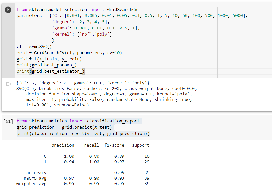
accfrom sklearn.model_selection import GridSearchCV
parameters = {'C': [0.001, 0.005, 0.01, 0.05, 0.1, 0.5, 1, 5, 10, 50, 100, 500, 1000, 5000],
'degree': [2, 3, 4, 5],
'gamma':[0.001, 0.01, 0.1, 0.5, 1],
'kernel': ['rbf','poly']
}
cl = svm.SVC()
grid = GridSearchCV(cl, parameters, cv=10)
grid.fit(X_train, y_train)
print(grid.best_params_)
print(grid.best_estimator_)from sklearn.metrics import classification_report
grid_prediction = grid.predict(X_test)
print(classification_report(y_test, grid_prediction))
SVM – Regression:
import numpy as np
import matplotlib.pyplot as plt
import pandas as pd
dataset = pd.read_csv('Position_Salaries.csv')dataset.head()
dataset.tail()
dataset.columns
dataset.shape
dataset.describe()
print(str('Any missing data or NaN in the dataset:'),dataset.isnull().values.any())
dataset.info()X = dataset.iloc[:, 1:2].values
y = dataset.iloc[:, 2].valuesy = y.reshape(-1,1)from sklearn.preprocessing import StandardScaler
sc_X = StandardScaler()
sc_y = StandardScaler()
X = sc_X.fit_transform(X)
y = sc_y.fit_transform(y)from sklearn.svm import SVR
regressor = SVR(kernel = 'rbf')
regressor.fit(X, y)y_pred = regressor.predict([[6.5]])
y_pred = sc_y.inverse_transform(y_pred)
print(y_pred)plt.scatter(X, y, color = 'red')
plt.plot(X, regressor.predict(X), color = 'blue')
plt.title('Truth or Bluff (SVR)')
plt.xlabel('Position level')
plt.ylabel('Salary')
plt.show()
X_grid = np.arange(min(X), max(X), 0.01) #this step required because data is feature scaled.
X_grid = X_grid.reshape((len(X_grid), 1))
plt.scatter(X, y, color = 'red')
plt.plot(X_grid, regressor.predict(X_grid), color = 'blue')
plt.title('Truth or Bluff (SVR)')
plt.xlabel('Position level')
plt.ylabel('Salary')
plt.show()
End Notes:
In this article, we have discussed Support Vector Machine: Machine Learning and its types, Maximum margin classifier, Support Vector Classifier, Kernel trick & its types, parameters essential, a summary of SVM, advantage, and disadvantage, application of SVM, and lastly cheatsheet too. In the last session, I have included Python code for SVM step by step for a simple dataset, by doing the slight modification, we can adopt this coding for all types of the dataset, both for classification and regression.
Did you find this article helpful? Please share your opinions/thoughts in the comments section below. Learn from mistakes is my favorite quote, if you found anything wrong too, just highlight it, I am ready to learn from the learners like you people.
About me in short, I am Premanand.S, Assistant Professor Jr and a researcher in Machine Learning. Love to teach and love to learn new things in Data Science. Mail me for any doubt or mistake, [email protected], and my Linkedin https://www.linkedin.com/in/premsanand/
Happy learning!!
The media shown in this article are not owned by Analytics Vidhya and are used at the Author’s discretion.


Thank you for writing such an awesome post. Would be really helpful if you could also explain the maths behind how the cost optimization would happen here.
it was really good and helped me to understand the concepts
Movie super hai,.......hit and block buster.....100 days pakka
Movie super hai,.......hit and block buster.....100 days pakka
First of all, this is really great article, with quality content. But it would make it even better if you fixed the grammar on this article. Otherwise, awesome job. Sincerely, Antonio
very very helpful.. thank you very much for this detailed explanation of the concepts and maths behind this
Thanks Premanand, this is in detail and helpful. One question, what is the purpose of using >> dataset = pd.get_dummies(dataset, prefix_sep='sex') << get_dummies in the preprocessing step, i don't see any purpose in this dataset or am i missing any ?
Well structured and informative article! Appreciate it.