This article was published as a part of the Data Science Blogathon
Introduction
This is the second article of the series on ‘Traversing the Trinity of Statistical Inference’. In this article, we’ll discuss the concept of confidence intervals. Before moving to the concept, we’ll take a slight detour and revise the ideas discussed in the previous article of this series.
We started with the example of a beverage company that is interested in knowing about the proportion of people who prefer tea over coffee. We stepped into the shoes of a statistician and began analyzing our experiment. The experiment involved surveying a group of 850 people (n = 850) and noting down their preference in the binary system of 0 (indicating preference of coffee) and 1 (indicating preference of tea). We defined a series of random variables X1, X2, …, Xn that follow a Bernoulli distribution to model our experiment.
We then explored certain basic properties of Xi and then introduced the idea of estimation. The sample-mean estimator (calculated as the average of our observations) was used for estimation and its properties were discussed in the light of the Law of Large Numbers (LLN) and the Central Limit Theorem (CLT). We concluded by evaluating the performance of our estimator through various metrics including bias, efficiency, quadratic risk, consistency, and asymptotic normality.
Now that we have familiarised ourselves with the fundamentals of estimation, we can take a step ahead and explore the second pillar of the realm of statistical science- Confidence Intervals. The purpose of confidence intervals, in layperson terms, is to create error bars around the estimated value of an unknown parameter. So, there are two aspects of a confidence interval:
- Confidence: It indicates the level of surety we wish to attain
- Interval: It indicates a range of values that our estimator can take.
In more definite terms, we wish to create an interval for our estimator such that the probability that the true parameter lies in that interval is fixed. And as we change that probability we increase or decrease the size of the interval. Here, we are trying to answer the following questions:
“Is there a range of possible outcomes that the estimate can take depending upon how confident we want to be? What is that range?” Let’s begin!
Topics:
A) Notation & Basic Properties of the Gaussian distribution
B) Asymptotic Normality of the Sample Mean Estimator
C) A General Notion for Confidence Intervals
D) Deriving the Asymptotic Confidence Intervals for the Sample Mean Estimator
E) Plug-in Method and the Frequentist Interpretation
F) Conservative Bound Method
G) Quadratic Method
A) Notations & Basic Properties of the Gaussian distribution
This section will revise a few basic properties and notations related to the normal/Gaussian distribution. These elements will play a critical role while deriving the confidence intervals.
1) Linear transformation of a Gaussian distribution: Let X follow a Gaussian distribution with mean µ and variance σ2. Suppose we are given a random variable Y that is a linear transformation of X such that:

Then, the distribution of Y will also be a gaussian with the mean (aµ + b) and variance (a2σ2).
2) Property of standardization: We have discussed the idea of standardization in the previous article of this series. Here, we’ll try to look at the process of standardization for the Gaussian distribution. Let X follow a Gaussian distribution with mean µ and variance σ2. Then, the standardized
form of X will follow a standard normal distribution i.e., a Gaussian with mean 0 and variance 1. Mathematically,

Here, the symbol Z has been used, which is the conventional notation for the standard Gaussian distribution.
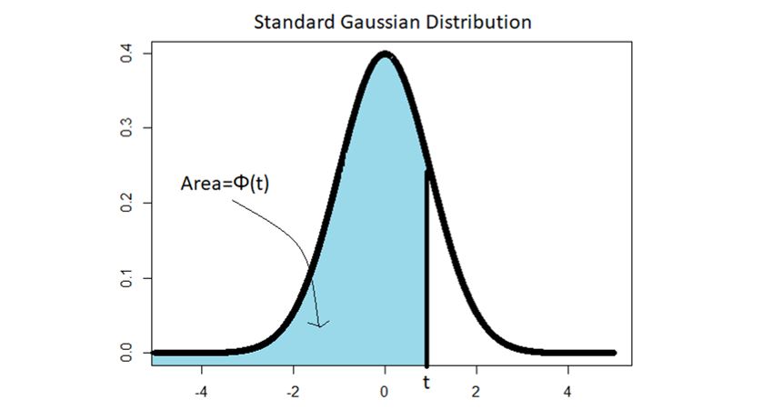
3) Cumulative Distribution Function (CDF) of a Gaussian Distribution: If Z follows a standard Gaussian distribution, then the following notation is used the CDF (the probability that Z is lesser than or equal to some number t) of Z:

Using this notation (and the property of standardization), we can obtain the CDF of any random variable X that follows a Gaussian distribution with mean µ and variance σ2:

Graphically, Φ(t) denotes the area below the standard Gaussian curve between -infinity and t. That is,
4) Quantiles of a Gaussian Distribution and its properties: If,

Where Φ-1 is the inverse of the CDF of the Gaussian. Essentially, Φ-1(x) gives a value t such that the area below the standard Gaussian curve between -infinity and t is equal to x. We define the quantiles of the gaussian as follows:

The value of q(x) can be easily computed using any statistical software.
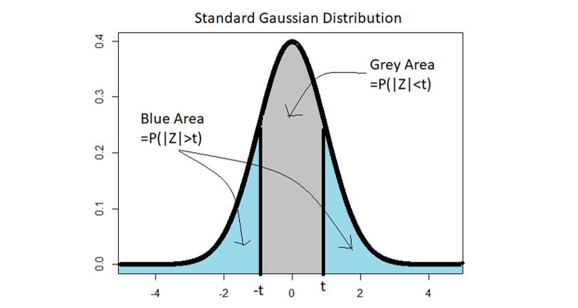
5) Symmetry: The Gaussian distribution is symmetric about its mean. So, the standard distribution is symmetric about 0, giving us a bunch of new properties (assuming t > 0):
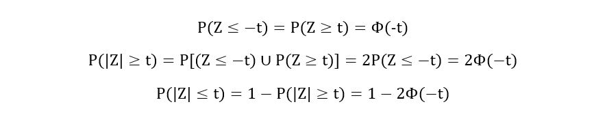
Graphically,
How are all these properties going to be useful to us? These properties will be relevant in the context of the asymptotic normality of the sample mean estimator, which has been discussed in the next section.
B) Asymptotic Normality of The Sample Mean Estimator
The application of the Central Limit Theorem (CLT) on the sample mean estimator gave us the following result:

It shows that the standardized version of the sample mean estimator converges (“in distribution”) to the standard Gaussian distribution. This property of estimators was called asymptotic normality. In fact, by using the properties of normal distribution, we can also conclude that the same mean estimator itself follows a normal distribution:
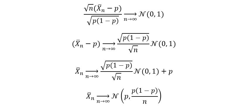
Property used: If X follows a Gaussian distribution with mean µ and variance σ2, then aX + b follows a normal distribution with mean aµ + b, and variance a2σ2. Let’s talk about this asymptotic normality more. In general, an estimator (or equivalently an estimate) θ-hat for parameter θ is said to exhibit asymptotic normality if:

Where σθ2 is referred to as the asymptotic variance of the estimator θ-hat.
Although not of much relevance, we can use the above definition (and properties of gaussian distribution), obtain the asymptotic variance of our sample mean estimator as follows:

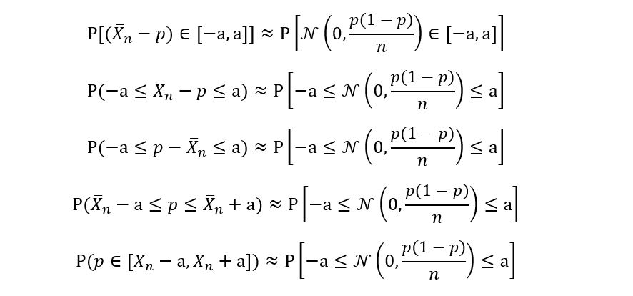
Thus the asymptotic variance of p-hat is p(1 – p). You might be wondering how is all this related to the idea of confidence intervals? Asymptotic normality allows us to garner information about the distribution of the sample mean estimator. Since we know that the above function of the sample mean estimator follows a gaussian distribution for large sample sizes, we can calculate the probability that the following function (of the sample mean estimator) lies between a certain interval A. Mathematically, we can say that (for large sample size):

Generally, it’s easier to play around with the following form:

This is like the core equation of this entire article. All new concepts will be built upon this equation.
C) A General Notion for Confidence Intervals
First, we’ll talk about a general notion (mathematically of course) of confidence intervals. We’ll then apply this notion to our example, mix it up with asymptotic normality, and develop something spicy.
Let Y1, Y2, …, Yn be some independent and identically distributed random variables with the following statistical model:

We introduce a new variable called α such that α ∈ (0, 1). Our goal is to create a confidence interval 𝕀 for the true parameter θ such that the probability that θ lies in 𝕀 is more than or equal to 1 – α. Mathematically,

Where 1 – α is called the level for the confidence interval 𝕀. You might be wondering, why I’ve taken 1 – α as the level instead of just some other α. You can, it’s not mathematically incorrect. It’s just that the notation works that way (probably due to some abstract reasons). Another important note, α is a deterministic quantity since its value is independent of the sample that we’ve taken. We can fix α to be any value of our choice. So, if the beverage company asks us to find a 90% confidence interval, we want to get a confidence interval 𝕀 for the true parameter p such that the probability
that p belongs to 𝕀 is more than or equal to 90% (or 0.9):

In other words, we fix our confidence interval at α = 0.10 and compute the confidence interval accordingly. Now, it won’t be easy for us to create confidence intervals for finite sample sizes. This is because the information about the distribution of the sample mean estimator is given by the Central Limit Theorem, which assumes large sample sizes (n approaches infinity). So instead of finite confidence intervals, we introduce asymptotic confidence intervals, which are defined as follows:

(For n > 30, we may assume n approaches infinity in most cases.) Throughout the rest of this article, whenever we are talking about confidence intervals, we shall always refer to asymptotic confidence intervals only.
The confidence intervals that we are describing for our example are two-sided because we are not interested in an upper or lower boundary that limits the value of our true parameter. On the other hand, in a one-sided confidence interval, our goal is to obtain a tight upper or lower bound for the true parameter. For instance, if we are interested in determining the mean concentration of toxic wastes in a water body, we don’t care about how low the mean could be. Our focus would be to determine how large the mean could be i.e., finding a tight upper bound for the mean concentration of the toxic wastes. This article shall restrict our discussion to two-sided confidence intervals as they are more relevant to our example. Why two-sided confidence interval for our example? Because we are not interested in overestimating or underestimating the true parameter p. Our focus is simply to find an interval that contains p with a certain confidence/level.
A two-sided confidence interval is generally symmetric about the estimator that we are using to determine the true parameter. In most cases, if θ-hat is our estimator for θ, then the two-sided confidence interval for θ (particular to our estimator) is represented as:

Where a is some quantity that we don’t know (but
will find later!). In our example, the confidence interval is described as follows:


And for the rest of the article, our goal will be to determine ‘a’.
Just a few concluding questions:
- What are the variables on which our confidence interval 𝕀 would depend upon?
𝕀 is going to depend upon the level 1 – α, the sample size n, and the value of the estimator θ-hat. So different estimators yield different confidence intervals. - Does the confidence interval depend upon the true parameter?
The answer is no. This must seem obvious: if 𝕀 was dependent on θ, then we wouldn’t have been able to calculate it. Hence, consider this as a rule of thumb: “Confidence intervals must be independent of the true parameter we are trying to estimate”. - The last question for this section: Is the confidence interval random or deterministic?
(Think….) The answer will be discussed later.
D) Deriving the Asymptotic Confidence Intervals for the Sample Mean Estimator
Now that we are well versed with the general notion and associated terminologies, we can start constructing the confidence interval for our example:
First, bring in equation 1 (that we obtained in section B) and define a suitable interval A:

We let A be the following interval:

Where a is some constant. Why this interval only? Because the above interval gives equation 1 a special form:
Does the LHS seem familiar? Remember equation 3?

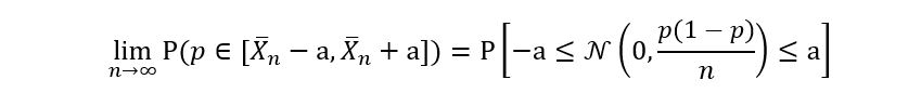
The LHS of equation 3 and equation 4 are the same! But what about the limit? Equation 3 has been derived from the CLT, which says large sample sizes. So, the limit is always there i.e., equation 4 can be rewritten as:
Comparing RHS of equations 3 and 4 gives us:

Now, we shall use the properties of the gaussian distribution to compute the LHS of the above equation:
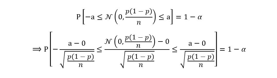
Using property 2 of Gaussian distributions i.e., standardizing the distribution to get the standard gaussian Z, we obtain the following equation:
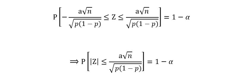
Recall that by the property of symmetry of the standard gaussian, we have,

Using this property, we get:
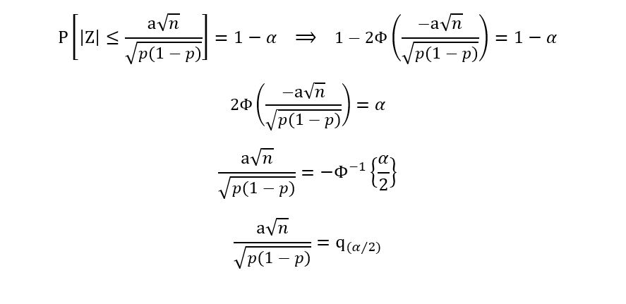
Recall the definition of quantiles of the gaussian distribution: q(α/2) denotes the αth/2 quantile. Thus, we obtain:

So, finally, we’ve obtained an expression for a! Let’s substitute this expression for ‘a’ in equation 2:
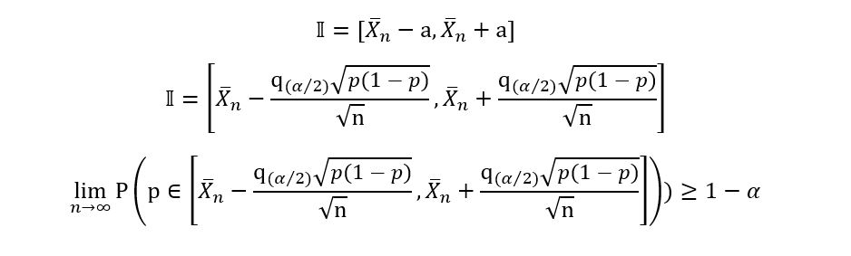
So, are we done? Not yet. Recall that the confidence interval cannot depend upon the true parameter p, which is not seen in the above expression. So, now we have another problem: remove the dependency of 𝕀 on p. The question is how? Well, there are 3 ways to resolve this problem.
E) Plug-in Method and the Frequentist Interpretation
The first method, which is possibly the simplest involves replacing the true parameter p in the expression for 𝕀 with the value of the estimator p-hat i.e., replace p with the sample mean. This gives us the following results:
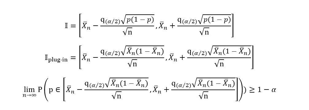
Yes, we’ve obtained a confidence interval! We’ll now plug in some real values and calculate 𝕀 for our example. Recall that from our survey we found out that 544 people prefer tea over coffee, while 306 people prefer coffee over tea.

So, now we compute:
- The 90% plug-in confidence interval for the proportion of people that prefer tea over coffee.
- The 95% plug-in confidence interval for the proportion of people that prefer tea over coffee.
Let’s solve these problems:
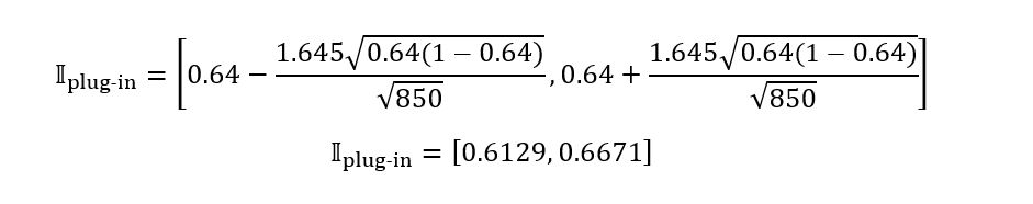
1) 90% plug-in confidence interval implies 1 – α = 0.90, giving us α=0.10. Using any statistical software, we can obtain that:

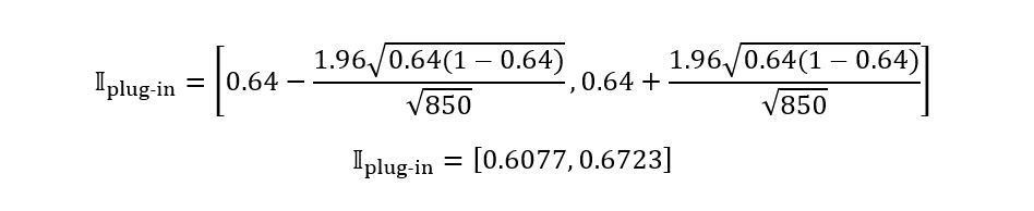
Substituting all these results in the expression
for 𝕀plug-in,
we obtain:
2) 95% plug-in confidence interval implies 1 – α = 0.95, giving us α=0.05. Using any statistical software, we can obtain that:

Substituting all these results in the expression for 𝕀plug-in, we obtain:
Observation: 𝕀plug-in for 95% confidence is larger than 𝕀plug-in for 90% confidence. This makes sense. The more we want to be confident about our parameter lying in an interval, the more is going to be the width of the interval. Before proceeding further with our discussion of the other methods, I find it very important to put forward a small question (that has a humongous answer):
What is the probability that the true p belongs to in the interval [0.6077, 0.6723]?
Answer: It’s not 0.95! That might seem confusing. We wanted to create an interval such that the probability that the interval contained p was at least 0.95. We did so and now we are saying that the probability is not 0.95! What’s the mystery?. Remember, I had asked you to find if confidence intervals are a random or deterministic quantity. The answer to that question was random since confidence intervals were dependent upon the estimator, which itself is a random quantity. In other words, the confidence interval for the parameter p depends upon the random sample we’ve chosen. If we had surveyed some other portion of Mumbai’s population, then the sample mean could have taken a different value, say 0.62 giving us a different confidence interval. Since 𝕀 was random, we could make statements such as:

But, once we plug in the true values, then the random 𝕀 assumes a deterministic value i.e., [0.6077, 0.6723]. It is no longer random. The probability that the true p belongs to this interval can be only 1 (if true p is some number that lies between 0.6077 and 0.6723) or 0 (if true p is some number that does not lie between 0.6077 and 0.6723). Mathematically,
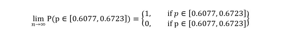
There’s no other probability that’s possible. We are calculating the probability that one deterministic quantity lies in another deterministic quantity. Where’s the randomness? Probabilistic statements require randomness, and in the absence of randomness, the statements do not make much sense.
It’s like asking what’s the probability that 2 is between 1 and 3? Of course, 2 is between 1 and 3, so the probability is 1; it’s a sure event. What’s the probability that 2 is between 3 and 4? Of course, 2 is not between 3 and 4, so the probability is 0; it’s an impossible event. Well, you might think we are back to square 1 since these intervals don’t make sense. What’s the use of that math we did? That’s because we still haven’t understood the interpretation of confidence intervals. (The mystery increases…)
So, how do we interpret 𝕀? Here, we shall discuss the frequentist interpretation of confidence intervals. Suppose we observed different samples i.e., we went across Mumbai surveying several groups of 850 people. For each sample, we’ll construct a 95% confidence interval. Then the true p will lie in at least 95% of the confidence intervals that we created. In other words, 95% is the minimum proportion of confidence intervals that contain the true p. Now that’s randomness. And that’s why we can make probabilistic statements here.
F) Conservative Bound Method
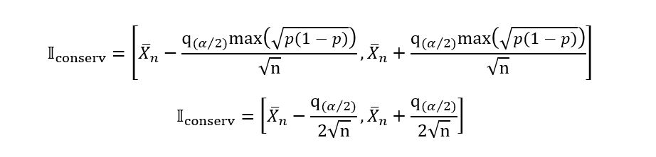
In this method, we replace the occurrence of p with the maximum value that the function of p can take. This method may not apply in many situations, but in our case, it works well. The expression we obtained for 𝕀 was:

The function that depends on p (that we want to modify to make it independent of p) is:

Here we replace the above function with its maximum value. How does that work? Remember that the probability that p belongs to 𝕀 must be at least 1 – α. So, if we substitute the maximum value of the above function, we’ll obtain the maximum width of the confidence interval, which does not really affect our probability of ‘at least 1 – α’. That’s why is called the conservative bound method. In fact, conservative confidence intervals have a higher probability of containing the true p because they are wider. So, we are interested in obtaining:

The maximum value can easily be found by using calculus. But instead, I’ll use the graphical approach as it’s more intuitive. The graph for sqrt(p*(1 – p)) is shown below:
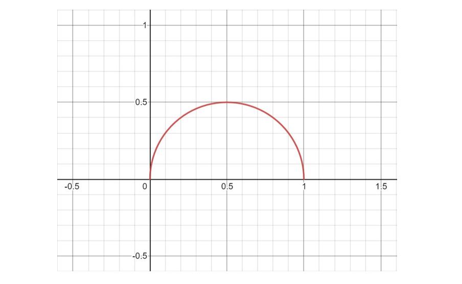
It can be seen that sqrt(p*(1 – p)) is maximised for p = 0.5, and the maximum value of the function is 0.5. Substituting all this in the expression for 𝕀 we obtain,
Thus, we have obtained the conservative confidence interval for our example. We shall now solve the following problems:
Compute:
- The 90% conservative confidence interval for the proportion of people that prefer tea over coffee.
- The 95% conservative confidence interval for the proportion of people that prefer tea over coffee.
Let’s solve these problems:
1) 90% conservative confidence interval implies
1 – α = 0.90, giving us α=0.10. Using any statistical software, we can obtain
that:

Substituting all these results in the expression
for 𝕀conserv,
we obtain

2) 95% conservative confidence interval implies
1 – α = 0.95, giving us α=0.05. Using any statistical software, we can obtain
that:

Substituting all these results in the expression
for 𝕀conserv,
we obtain:

Notice that the conservative confidence intervals are wider than the plug-in confidence intervals.
G) Quadratic Method
We shall now discuss the final method, which is possibly the hardest of all three. Although it generally gives good results (in terms of narrower confidence intervals), the process of calculating the intervals is much longer. The idea is as follows:
1) We assume that the true p belongs to 𝕀:

This gives us a system of two inequalities:
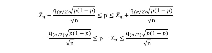
The above inequalities can also be represented as:

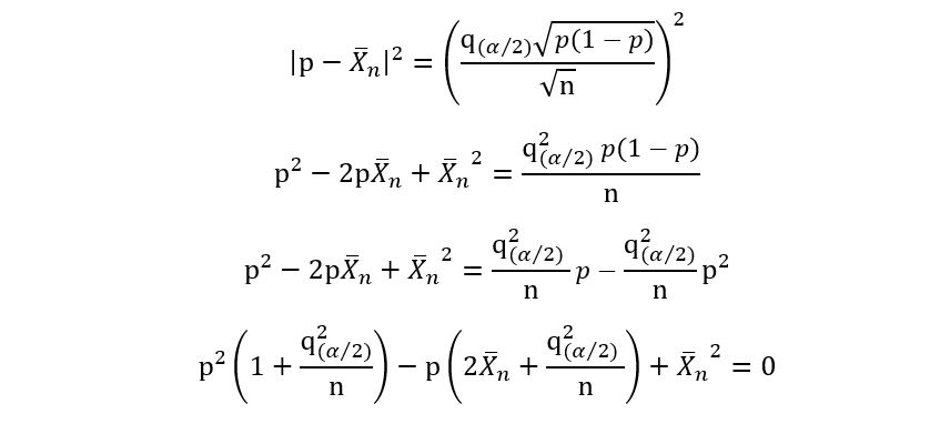
2) We square the above expression, which gives us:

We replace the ‘≤’ sign with ‘=’ sign and open the brackets to get the following quadratic equation:
3) We solve the above quadratic equation to get two solutions which shall be the lower and upper limits of the ‘solved’ confidence interval. Using the quadratic equation,
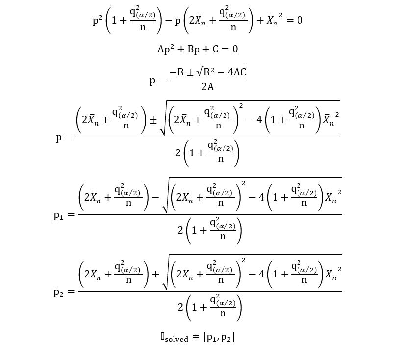
Yes, the solved confidence interval is that long-expression, which I cannot even fit in a single line. As I said, the interval is narrower, but the process is longer. We shall now solve the following problems:
Compute:
- The 90% solved confidence interval for the proportion of people that prefer tea over coffee.
- The 95% solved confidence interval for the proportion of people that prefer tea over coffee.
Let’s solve these problems:
1) 90% solved confidence interval implies 1 – α = 0.90, giving us α=0.10. Using any statistical software, we can obtain that:

Instead of using that long formula, we’ll obtain
a simple quadratic and solve it using any quadratic equation calculator:
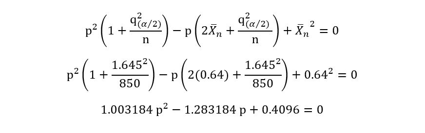
Solving, the above equation, we obtain:

2) 95% solved confidence interval implies 1 – α = 0.95, giving us α=0.05. Using any statistical software, we can obtain that:

Instead of using that long formula, we’ll obtain a simple quadratic and solve it using any quadratic equation calculator:
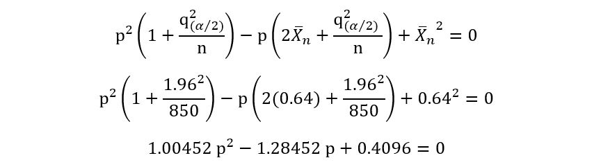
Solving, the above equation, we obtain:

Notice that the solved confidence intervals are narrower than the plug-in confidence intervals, but with a difference of only about 0.0001. So, it’s better but the magnitude of complexity is much more than the improvement attained.
This concludes our discussion on confidence intervals. The next and the final article of this series will describe the process of hypothesis testing. Unlike estimation and confidence intervals that gave results in numerical format, hypothesis testing will produce results in a yes/no format. It’s going to be a very exciting and challenging journey ahead!
Conclusion
In this article, we continued with our statistical project and understood the essence of confidence intervals. It’s important to note that we took a very basic and simplified example of confidence intervals. In the real world, the field of confidence intervals is vast. Various probability distributions require a mix of several techniques to create confidence intervals. The purpose of this article was to not only see confidence intervals as a mix of theory and math but also to make us feel the idea. I hope you enjoyed reading this article!
In case you have any doubts or suggestion, do reply in the comment box. Please feel free to contact me via mail.
If you liked my article and want to read more of them, visit this link. The other articles of this series will be found on the same link.
Note: All images have been made by the author.
About the Author

Image by Author
I am currently a high school student, who is deeply interested in Statistics, Data Science, Economics, and Machine Learning. I have written two data science research papers. You can find them here.
The media shown in this article are not owned by Analytics Vidhya and are used at the Author’s discretion.


