This article was published as a part of the Data Science Blogathon
Introduction
Deep neural networks are very fascinating and it produces magic as we try to predict something, maybe with images or texts. In the past 10 years, there has been a major improvement in deep learning, especially when it comes to Image recognition. Many researchers have been trying to develop newer models every week to improve the existing system’s accuracy.
Challenges in building Neural Networks
One of the major challenges included how deep networks could be built. Theoretically, it sounds cool to build deeper networks but in reality, it encounters a problem called degradation. It is the problem of the increase in the training error as deeper layers are constructed. This hurts our accuracy a lot. One another problem of building deeper networks includes the vanishing gradient descent. This happens in the backpropagation step, as we know in the neural networks we need to adjust weights after calculating the loss function.
While backpropagating, we follow the chain rule, the derivatives of each layer are multiplied down the network. When we use a lot of deeper layers, and we have hidden layers like sigmoid, we could have derivatives being scaled down below 0.25 for each layer. So when n number of layers derivatives are multiplied the gradient decreases exponentially as we propagate down to the initial layers.
As told earlier when we go very deep into a network we get blocks that have learned a lot and when we add deeper blocks to it tends to be just an identity mapping of the earlier block that is it is just the same as the earlier block. Degradation results suggest that there are difficulties in learning this identity mapping. To solve these problems we come across the ResNet paper. These are residual networks stacked together that allow us to build deep networks without degradation or vanishing gradient descent.
 Train and Test error visualized on 56 and 34 layers plain model (https://arxiv.org/pdf/1512.03385.pdf)
We may think that it could be a result of overfitting too, but here the error% of the 56-layer network is worst on both training as well as testing data which does not happen when the model is overfitting.
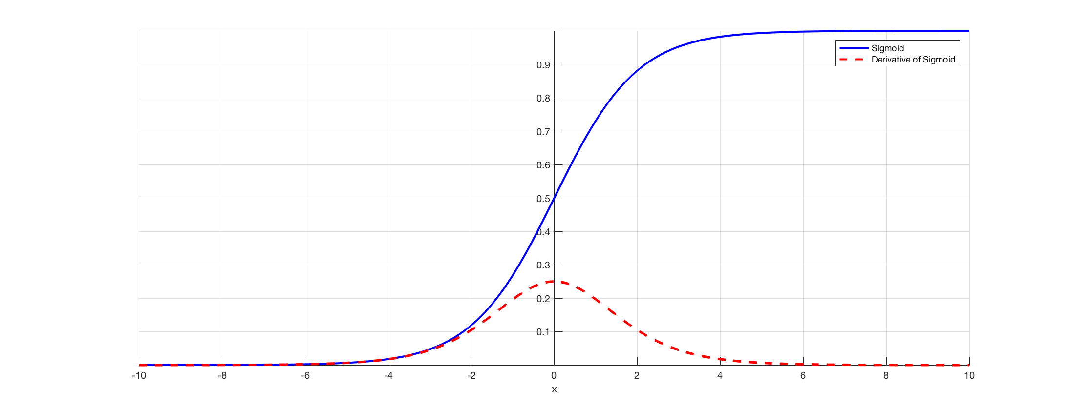 Derivative of sigmoid layers (https://towardsdatascience.com/the-vanishing-gradient-problem-69bf08b15484)
We can see the derivative of the sigmoid function is from a value of 0 to 0.25 which brings down the value and when we multiply the chain of such values as deeper layers we go, we end up with a very small value which affects weight updation through our loss function.
How does ResNet work?
Let us now understand how ResNet works. Here, we have something called Residual blocks. Many Residual blocks are stacked together to form a ResNet. We have “skipped connections” which are the major part of ResNet. The following image was provided by the authors in the original paper which denotes how a residual network works. The idea is to connect the input of a layer directly to the output of a layer after skipping a few connections. We can see here, x is the input to the layer which we are directly using to connect to a layer after skipping the identity connections and if we think the output from identity connection to be F(x). Then we can say the output will be F(x) + x.
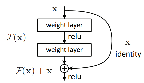
Residual Learning – Building block(https://arxiv.org/pdf/1512.03385.pdf)
One problem that may happen is regarding the dimensions. Sometimes the dimensions of x and F(x) may vary and this needs to be solved. Two approaches can be followed in such situations. One involves padding the input x with weights such as it now brought equal to that of the value coming out. The second way includes using a convolutional layer from x to addition to F(x).
This way we can bring down the weights same dimensions of that coming out. When following the first way, the equation turns to be F(x) + w1.x. Here w1 is the additional parameters added so that we can bring up the dimensions to that of output coming from the activation function. The skip connections in ResNet solve the problem of vanishing gradient in deep neural networks by allowing this alternate shortcut path for the gradient to flow through.
It also helps the connections by allowing the model to learn the identity functions which ensures that the higher layer will perform at least as good as the lower layer, and not worse. The complete idea is to make F(x) = 0. So that at the end we have Y = X as result. This means that the value coming out from the activation function of the identity blocks is the same as the input from which we skipped the connections.
Comparison of ResNet with Plain Networks
Now let us compare the ResNet with the plain networks. According to the deep learning course, Andrew NG has told us that one of the main benefits of ResNet is how they perform in training errors. If we see the plain networks, as we increase the layers there is a decrease in train error, but after few layers, the error goes back increasing. This is why deploy methods like early stopping. But this behavior is solved when it comes to ResNet and as layers are increasing the error only tends to decrease and don’t increase. The authors of the ResNet paper have also given us the comparison between how plain networks and ResNet works over 18 and 34 layers and we can see that the ResNet gives us lesser error compared to plain networks.
 Plain vs ResNet (https://arxiv.org/pdf/1512.03385.pdf)
ResNet Architecture
Now, let us understand the architecture of the ResNet models. We have a comparison here of 34 layered plain and ResNet models.

Architecture of ResNet34 (https://arxiv.org/pdf/1512.03385.pdf)
We can see here, initially, we have our image being passed through a 7 * 7 filter with a stride of two with 64 channels. We can imagine that if we had an image of 300 * 300 * 64 then after the first operation, it would have been changed to 150 * 150 * 64, after applying the formula,
- Input: n X n
- Padding: p
- Filter size: f X f
- Output: ((n+2p-f)/s+1) X ((n+2p-f)/s+1)
Next, we perform a 3 * 3 max-pooling with stride 2 and we end up 75 * 75 * 64 as the output pooling layer. Then we can see there is a 3 * 3 filter with 64 channels as convolution operation is being performed two times, but these two layers are skipped connections as they are a residual block. The same occurs again two times and we use the skipped connections to form the residual block. Now, we can see there is 128 instead of 64 and we cannot directly pass input to the activation function output from the 128 layers because of dimension mismatch. In such cases, as we discussed earlier, we apply convolutional operation or padded weights to make dimension equal. In other cases, we have an identity block and the connections are direct from input and appended to the output. This is carried out as shown in the architecture and the end, we have an average pooling operation and features are extracted out. If we want to perform this on the CIFAR-10 dataset, we must remove the last layer and apply a dropout and then add a linear layer to get the probability of 10 features.
The following is the architecture of the 18,34,50,101 and 152 layered ResNet model. All of them work the same way as explained above.
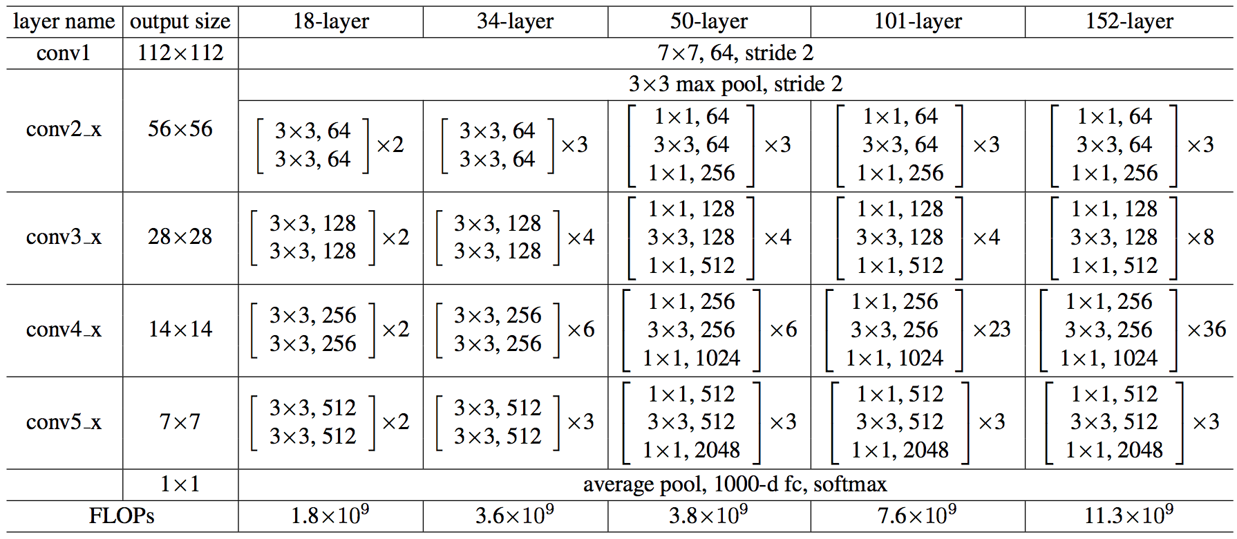 Architecture of ResNet (https://arxiv.org/pdf/1512.03385.pdf)
ResNeXt Model
We also have another model called the ResNeXt, which was introduced by scientists at Facebook and uses the same idea as the ResNet. Except it has a cardinality factor of 32, which means there are 32 paths and the convolution operation is divided across. the main idea is that when doing so, we have matrix multiplication of 4 * 4 which is faster and at the end, we can make out the same number of parameters as the ResNet model. The following diagram compares ResNet and ResNeXt model and will help you understand how it works,
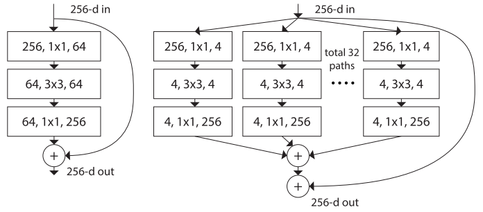
Working of ResNext (https://arxiv.org/pdf/1611.05431.pdf)
Analysis of CIFAR-10 on ResNet models
I carried out an analysis on the CIFAR-10 dataset to see how different ResNet models worked and to see if whatever we discussed, in theory, held. I used the idea of transfer learning, where I had the pre-trained models directly implemented from PyTorch using the touchvision.models module. The basic abstraction for each used in code as shown:
resnet18 = models.resnet18()
resnet34 = models.resnet34()
resnet50 = models.resnet50()
resnext50_32x4d = models.resnext50_32x4d()
resnet101 = models.resnet101()
resnet152 = models.resnet152()
You can refer to this code from the PyTorch torchvision documentation.
The results of the implementation are as follows:
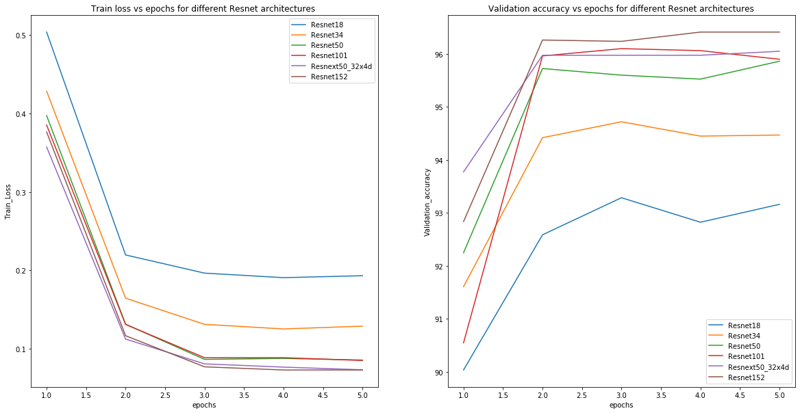
We can see that as the layers increases, there has been a decrease in the training loss and an increase in the accuracy on the validation set. The ResNet with 18 layers suffered the highest loss after completing 5 epochs around 0.19 while 152 layered only suffered a loss of 0.07. Also, accuracy came around 96.5 for ResNet152 while around 93.2 for ResNet18. We can compare both ResNet50 and ResNeXt50 with cardinality as 32 and see that ResNeXt has performed better over the ResNet50 model. Further, we can analyze the test accuracy of each model and see that deeper models are performing better. Also, note that these are results on 5 epochs and we could improve it to more extent by using different regularization techniques and running for more epochs.
.png)
Test accuracy across different ResNet models.
References
1. https://arxiv.org/pdf/1512.03385.pdf (Original ResNet Paper)
2. https://arxiv.org/pdf/1611.05431.pdf (Original ResNeXt Paper)
3. https://towardsdatascience.com/the-vanishing-gradient-problem-69bf08b15484 (Vanishing gradient problem explained)
4. https://www.mygreatlearning.com/blog/resnet/ (Blog on ResNet)
5. https://pytorch.org/vision/stable/models.html (Torchvision models)
6. https://jovian.ai/learn/deep-learning-with-pytorch-zero-to-gans (Deep Learning Course)
The Thumbnail image is taken from: https://unsplash.com/photos/0E_vhMVqL9g
Conclusion
I have also created a custom ResNet model by referring to Jovian’s Deep Learning course and the code is available on my Github profile. Feel free to play with it and build your own ResNet models.
The entire code for implementation and results can be obtained from my GitHub repo. I would be happy to contribute to projects related to Deep Learning and you can reach me at [email protected].
Linkedin: https://www.linkedin.com/in/siddharth-m-426a9614a/
The media shown in this article are not owned by Analytics Vidhya and are used at the Author’s discretion.
Siddharth M
23 Jun, 2021


