A Comprehensive Guide to Decision trees

Introduction

Decision trees are versatile machine learning algorithm capable of performing both regression and classification task and even work in case of tasks which has multiple outputs. They are powerful algorithms, capable of fitting even complex datasets. They are also the fundamental components of Random Forests, which is one of the most powerful machine learning algorithms available today.

By the end of the article, I assure you that you will know almost everything regarding decision trees. So let’s get started!

This article was published as a part of the Data Science Blogathon.

Training and Visualizing a Decision Tree

To get a stronghold on this algorithm, let’s us build one and take a look at a journey our algorithm went through to make a particular prediction. In this article, we will be using the famous iris dataset for the explanation.

Training

1. Importing iris dataset from sklearn.datasets and our decision tree classifier from sklearn.tree:

from sklearn.datasets import load_iris
from sklearn.tree import DecisionTreeClassifier

2. Initializing the X and Y parameters and loading our dataset:

iris = load_iris()
X = iris.data[:,2:]
y=iris.target

Here, X is the feature attribute and y is the target attribute(ones we want to predict).

3. Initializing a decision tree classifier with max_depth=2 and fitting our feature and target attributes in it.

tree_classifier = DecisionTreeClassifier(max_depth=2)
tree_classifier.fit(X,y)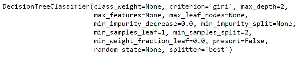

All the hyperparameters in this model are set by default;

max_depth is the longest path between the root node and the leaf node(we will see at the time of example below).

Visualizing

There are several ways of visualizing our trees:

1. Exporting decision trees to the text representation. It can be used while working on an application with UI(User Interface) or when we want to log information of model into a text file.

from sklearn.tree import export_text
txt_tree = export_text(tree_classifier)
print(txt_tree)

Hit Run to see the output

2. Using Plot_tree(requires matplotlib make sure to import it):

import matplotlib.pyplot as plt
from sklearn.tree import plot_tree
%matplotlib inline
fig = plt.figure(figsize=(25,20))
_ = plot_tree(tree_classifier, 
                   feature_names=iris.feature_names,  
                   class_names=iris.target_names,
                   filled=True)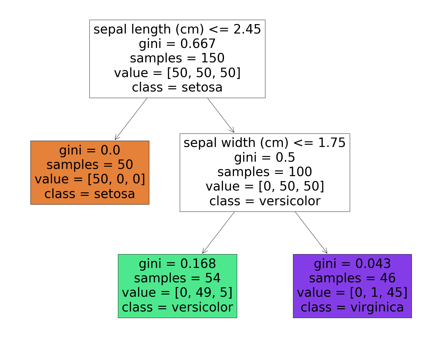

Here we can see that the longest path between the root node and leaf node is 2 which we had set at the time of model creation i.e max_depth.

Journey to the Predictions

Let’s see how the above decision tree makes its way to the predictions.

Suppose one day you are walking in a garden, and you find a beautiful iris flower and want to classify it.

Firstly, you will begin from the root node which is the top (depth 0): This node asks you a question whether the flower’s petal length is smaller than 2.45 or not? Here we suppose it is, then we move down to the root’s left child node which happens to be a leaf node(one with no child nodes), so it does not ask any further question: it simply looks at the prediction class for that node and our model predicts that the flower you found was Iris setosa.

Now suppose you find another flower, and this time the petal length is greater than 2.45 cm. So this time it moves towards the root’s right child node(depth 1), which is not a leaf node, and asks another question whether the petal width is smaller than 1.75 cm or not? If yes, your flower is most likely to be Iris versicolor. If no, your flower is most likely to be Iris virginica.

Simple!!

So one of the major features or we can say advantages of using a decision tree is that they require less data preparation. In fact, they do not need any kind of feature scaling at all.

Samples, values, and Gini?

So now you must be wondering, what do samples, values, and gini mean?

Samples:

Here we can say that a node’s samples attribute counts how many training instances it applies to. Let’s understand it with help of an example, suppose 100 training instances have a petal length greater than 2.45 cm(depth 1 right side ), and out of those 100, 54 have petal width smaller than 1.75 cm (depth 2, left).

Values:

A value attributes tell you how many training instances of each class this node applies to. For eg if we observe class “Versicolor” bottom left we have 0 Iris setosa, 49 Iris Versicolor, and 5 Iris Virginica.

Gini:

A node’s Gini attribute measures its impurity. A node is said to be pure when all training instances it applies belong to the same class. For example, we can see that in class Iris setosa gini appears to be 0  which means it is “pure”.

An equation to calculate the Gini score is given below:

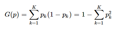
Let’s calculate the Gini score for class Iris Versicolor:

G(p) = 1 – (0/54)²  – (49/54)² – (5/54)² 

G(p)  = 0.168 (approx)

Interpretation of Model:

As we have seen here today, that decision trees are really powerful and their decisions are quite easy to interpret. These types of models are knowns as white-box models. In the near future, I will be uploading blogs about neural networks which are considered to be black-box models. In fact, neural networks help in getting great predictions and we can easily check the calculations they perform to give a prediction. But it is hard to explain why those predictions were made. For example, suppose a neural network says Elon musk appears to be in the picture, it is difficult to know what led to this prediction: It might have been eyes? or mouth? or nose? It is difficult to interpret that. But that is definitely not the case with decision trees they provide simple classification rules that we can apply manually if we want to.

Estimating Class Probability:

We can also estimate the probability that an instance belongs to a particular class. To calculate the probability what it does is, traverses to find the leaf node for a specific instance and then returns the ratio of an instance of the class in this node. For example, suppose we found a flower whose petal length is 4.5 cm long and 2 cm wide. So decision tree should output the following probabilities: 0 % for Iris setosa, 2.1 % for Versicolor, 97.8% for Iris virginica, and if you want to predict the class, it outputs class 2 because it has the highest probability.

tree_classifier.predict_proba([[4.5,2]])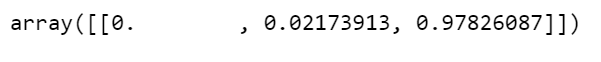

tree_classifier.predict([[4.5,2]])

Perfect !!

Grab a coffee before you go any further!

Image Source

Complexity

For making a prediction, we need to traverse the decision tree from the root node to the leaf. Decision trees are generally balanced, so while traversing it requires going roughly through O(log₂(m)) nodes. As we know that in each node we need to check only one feature, the overall prediction complexity is O(log₂(m)) which is independent of the number of features. Hence, our predictions are extremely fast, even with large training datasets. 

If we compare all features with all samples at each node the complexity will be of O(n x m log2(m)). If your training datasets are small you can speed up your training by presorting the data(set presort = True), but doing this in the case of larger datasets might slow it down.

CART Algorithm

Classification and regression tree (CART) algorithm is used by Sckit-Learn to train decision trees. So what this algorithm does is firstly it splits the training set into two subsets using a single feature let’s say x and a threshold t_x as in the earlier example our root node was “Petal Length”(x) and <= 2.45 cm(t_x). Now you must be wondering how does it choose x and t_x? It searches for a pair that will produce the purest subsets. Once the algorithm splits the training sets in two, it then splits the subsets with the same method and so on. This will stop when the max depth is reached (the hyperparameter which we set 2 earlier), or when it fails to find any other split that will reduce the impurity. There are a few other hyperparameters that control these stopping conditions, discussed in the regularization part.

Hyperparameters Regularizations

So when it comes to decision trees the thing is, it makes very few assumptions about training data (linear model assumes that the data you will be feeding will be linear). If you don’t constraint it, the tree will adapt itself to the training data, which will lead to overfitting. Such types of models are often called non-parametric models. Because the number of parameters is not determined before the training, so our model is free to fit closely with the training data.

To avoid this overfitting you need to constraint the decision trees during training. The regularizations of hyperparameters depend on the algorithm used, but you could at least set the maximum depth of the decision tree. This is can be controlled by the max_depth hyperparameter which we used earlier in the example its default value is None reducing the value of max_depth will regularize the model and hence avoid the risk of overfitting.

The few other hyperparameters that would restrict the structure of the decision tree are:

1. min_samples_split – Minimum number of samples a node must possess before splitting.
2. min_samples_leaf – Minimum number of samples a leaf node must possess.
3. min_weight_fraction_leaf – Minimum fraction of the sum total of weights required to be at a leaf node.
4. max_leaf_nodes – Maximum number of leaf nodes a decision tree can have.
5. max_features – Maximum number of features that are taken into the account for splitting each node.

Remember increasing min hyperparameters or reducing max hyperparameters will regularize the model.

Regression using Decision Trees

Yes, decision trees can also perform regression tasks. Let’s go ahead and build one using Scikit-Learn’s DecisionTreeRegressor class, here we will set max_depth = 5.

Importing the libraries:

import numpy as np
from sklearn.tree import DecisionTreeRegressor
import matplotlib.pyplot as plt
from sklearn.tree import plot_tree
%matplotlib inline

Initializing dataset:

dataset = np.array(
[[2,4],
 [3,9],
 [4,16],
 [5,25],
 [6,36],
 [8,64],
 [10,100],
 [12,144],
 [13,169]
])
X = dataset[:, 0:1].astype(int) 
y = dataset[:,1].astype(int)

Initializing model and fitting the data:

tree_regressor = DecisionTreeRegressor(max_depth=5)
tree_regressor.fit(X,y)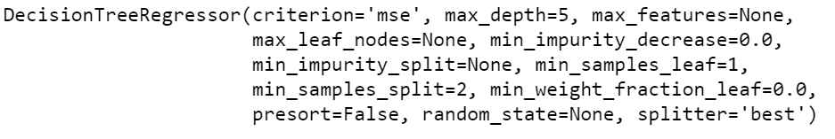

All the hyperparameters here are set by default.

Here also we will be using plot_tree to visualize the decision tree.

fig = plt.figure(figsize=(25,20))
_ = plot_tree(tree_regressor, 
                   filled=True)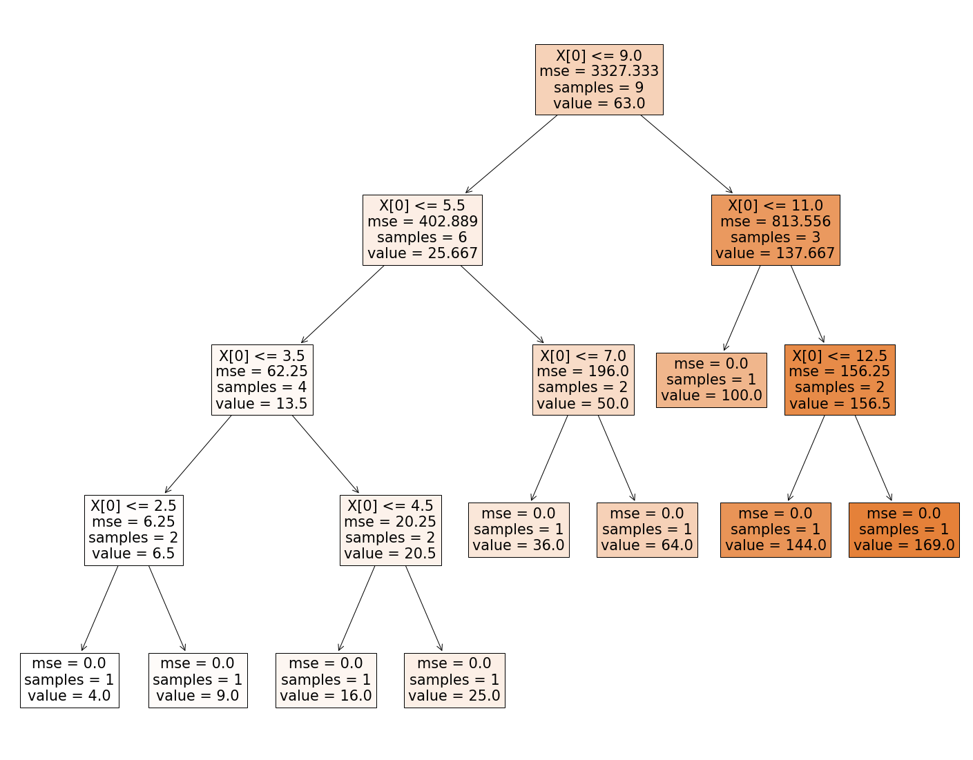

As we can see that, this tree looks kind of similar to the tree we built earlier. The difference is that instead of predicting the class in each node this time, it predicts a value. We are already aware of transversing the tree so we won’t be doing that here.

The Cart algorithm, here also works pretty much the same way, except that here instead of trying to minimizes the impurity while splitting it focuses on minimizing the MSE(Mean Square Error).

Decision Tree while performing the regression tasks is also prone to overfitting without any regularization which is definitely the case in our example.

Conclusion

Alright, So we wrap up with a comprehensive guide to the Decision tree here. At last, I would say that decision trees are really easy to use, understand and interpret. But the issue with decision trees is that they are extremely sensitive to minor variations in the training data. Actually, if train your model again on the same datasets you may get different results because the training algorithm used by Scikit-Learn is stochastic(Randomly selects a set of features), just set the random_state hyperparameter to get the same results on the same training datasets. The small variation issue in the decision tree can be countered by using Random Forests which we will be discussing in the upcoming blogs. Stay tuned!!

Frequently Asked Questions

The media shown in this article are not owned by Analytics Vidhya and are used at the Author’s discretion.

Karan Pradhan 28 Nov 2023