This article was published as a part of the Data Science Blogathon
Introduction
“Vision is an Art of Seeing what is invisible to others.” – Jonathan Swift
Computer Vision enables computers to see what is invisible to them and this technology has been evolved so much for humans to see things that are not even there. For example, a black and white version of a Colored Image.
There are many Computer Vision and Machine Learning Libraries that allow us to do this. Like: OpenCV, Korina, Scikit – Image, PIL, SimpleCV, PG Magic.
This is a series, we will be learning about the basic implementation and features of these libraries starting with OpenCV.
Table contents
- Image Theory
- I/O Image, Video, and Webcam
- Basic functions
- Resizing and Cropping Image
- Adding text to images
Before we get started with using computer vision, let us get familiar with the most basic understanding of an image.
The Image Theory
For a machine, an Image is interpreted as a two-dimensional matrix formed with rows and columns of pixels.
Pixel: here refers to the smaller to the smallest accessible part of an image.
Image Resolution: Image Resolution tells us the number of pixels in an image.
It is defined by the width and the height of an image
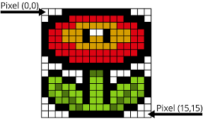
Some common types of image resolutions are :
- VGA (Video Graphics Array) : 640 X 480
- HD (High Definition ): 1280 X 720
- FHD (Full High Definition) : 1920 X 1080
- 4K : 3840 X 2160
Binary Image: A black and white image is called a binary image.
Why? As we know images are made of small elements/boxes in a black and white image, a box is either filled with black denoted by zero or it could be white denoted by 1.
Hence, it is referred to as Binary Image.
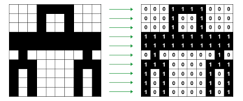
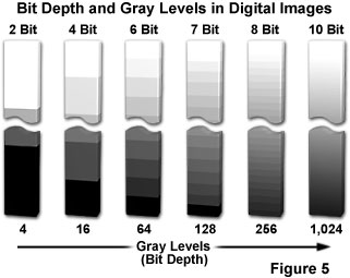
But these are not the usual black and white images that we see, they are more detailed.
That just means it has more levels.
Setting up the Environment
- Install Pycharm 3.7 as it works well with OpenCV,
- Open New Project and select Project Interpreter as 3.7
- Install OpenCV Library in Pycharm.
- Guide to Installing Packages in Pycharm
import cv2sou
Note: OpenCV released two python interfaces, cv, and cv2. cv2 is the latest version and we will be using the same.
I/O Images, Videos, and Webcam
We have imread() function in OpenCV to read images. But for that we need to create an image variable, let’s say ‘img’.
The imread() function will take the path of the image file that needs to be read as an argument.
(directly inserting path in imshow() needs double commas “ . “ )
Eg : img = cv2.imread(“Resources/lena.png”)
Syntax :
img = cv2.imread(“ path location of Image folder”)
OR ( this method of using path variable has single comas ‘ . ‘ )
path = ‘Resources/lena.png’
img = cv2.imshow(path)
Basic Functions
Converting to different colorspaces
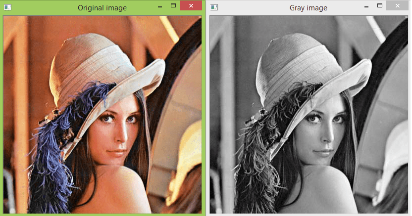
Using cvtcolor() function is used to convert an image into more than 150 color spaces.
Syntax :
img= cv2.cvtcolor( prev_img_object, colorspace)
Example :
#converts to gray colorspace
img=cv2.imread("Resource/lena.png")
imgGray=cv2.cvtcolor(img,COLOR_BGR2GRAY)
 cv2.imshow("Gray Image",imGray)
 cv2.waitKey(0)
Note: CONVENTIONALLY we use RBG, BUT in OpenCV, we write it as BGR.
Output after applying Gray Scale
Blur
The Gaussian Blur function is used to give blur effect to an image.
Syntax :
imgBlur = cv2.GaussianBlur(prev_img_object, (kernel size, Kernel Size) , sigma x)
# Kernel size can only be odd numbers
#Sigma x - controls variance of kernel applied on image
Example :
img = cv2.imread (“Resources/lena.png”)
imgGray= cv2.cvtcolor(img, COLOR_BGR2GRAY)
imgBlur = cv2.GaussianBlur(imgBlur, (7,7),0)
cv2.imshow(“Blur Image “ , imgBlur)
Output after Gaussian Blurr
Canny Edge Detector
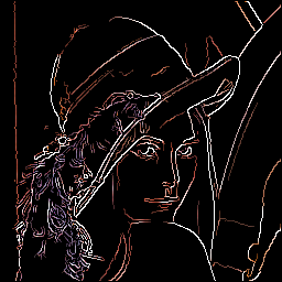
Canny Edge Detection is a technique used to extract the structural information, i.e. Edges. It takes grayscale image as input.
Syntax :
imgCanny = cv2.Canny(prev_img_obj, threshold 1 , threshold 2)
Example :
imgCanny = cv2.Canny(img,150,200)
Output for Canny Edge Detector
Image Dilation
It is a technique used to expand the pixels of an image along the edges. It is used to thicken the edges in the image to remove the gap in images.
Note: We will be dealing with kernel sizes – matrices, therefore, import NumPy.
The first step would be to define the kernel.
Syntax :
Kernel = np.ones( size1, size2)
#Where size 1 and size 2 are dimensions of matrix size 1 X size2
imgDialation = cv2.dilate( imgCanny, kernel , interactions =n)
Example :
kernel = np.ones( 5,5)      // ones - mean we want all the values of kernel to be 1
imgDialation = cv2.dilate( imgCanny, kernel , interactions =1)
-
Used imgCanny as prev object in image dilation as image dilation is applied on the Edges (Canny Edges)
-
The number of Iterations influences the thickness of the edges dilated.

Output for Dilation
Erosion – Complement to Dilation
Since erosion is the opposite of dilation, if we apply erosion to the dilated version of the image, we can get results similar to the Canny Edge version of the Image. Erosion computes the minimum area of a pixel over a given area.
Syntax :
imgEroded = cv2.erode( imgCanny, kernel , interactions =n)
Example :
imgEroded = cv2.erode( imgDilation,kernel , interactions =n)
cv2.imshow(“Eroded Image “ , imgEroded)

Output for Erosion
Resizing and Cropping
OpenCV Convention
.png)
Resizing Image
Note: To resize the image we need to know the current size of the image. For this, we use the shape function.
Finding the current size of the image :
Syntax :
print(img_name.shape)
Example :
img = cv2.imread(“Resources/lambo.png”)
cv2.imshow(“Original Image”,img

#checking the shape of image
print(img.shape)
Output :
|
Note: Here 462 is the height, 623 in Width, and 3 represents the RBG channels.
Resize Function is used to resize the image, it takes the new height and width as parameters.
Syntax :
ResizedImage = cv2.resize(orgninalimagename,(new height, new width))
Example :
imgResize = cv2.resize (img,( 300,200))
print(imgResize.shape)
| Output : |
Note: Here 200 and 300 are the new height and width respectively. |
Cropping Image
Image is an array of pixels, it is a matrix. So we don’t require any special OpenCV function, we can simply do that using matrix functions of Numpy.
Syntax :
imgCropped = img [ Start_height : End_height , start_width : end_width]
Note In Open Cv functions we write width first and then the height
Adding Text to Images
We use the function cv2.put Text() to add text to an image. It takes the text to be added, starts coordinates, font type, thickness, and the color of the text in BRG format and the scale – size of the text.
Syntax :
cv2.putText ( img_obj, “text_here”, (start coordinates) , cv2.Font_Type , scale , (B,R,G),Thickness)
Example :
cv2.putText ( img, “ OPENCV ”, (100,200) , cv2.Font_HERSHEY_COMPLEX, 1 , (255,0,0),2)
These are some of the fonts and scales available in OpenCV:
- FONT_HERSHEY_SIMPLEX = 0
- FONT_HERSHEY_PLAIN = 1
- FONT_HERSHEY_DUPLEX = 2
- FONT_HERSHEY_COMPLEX = 3
- FONT_HERSHEY_TRIPLEX = 4
- FONT_HERSHEY_COMPLEX_SMALL = 5
- FONT_HERSHEY_SCRIPT_SIMPLEX = 6
- FONT_HERSHEY_SCRIPT_COMPLEX = 7
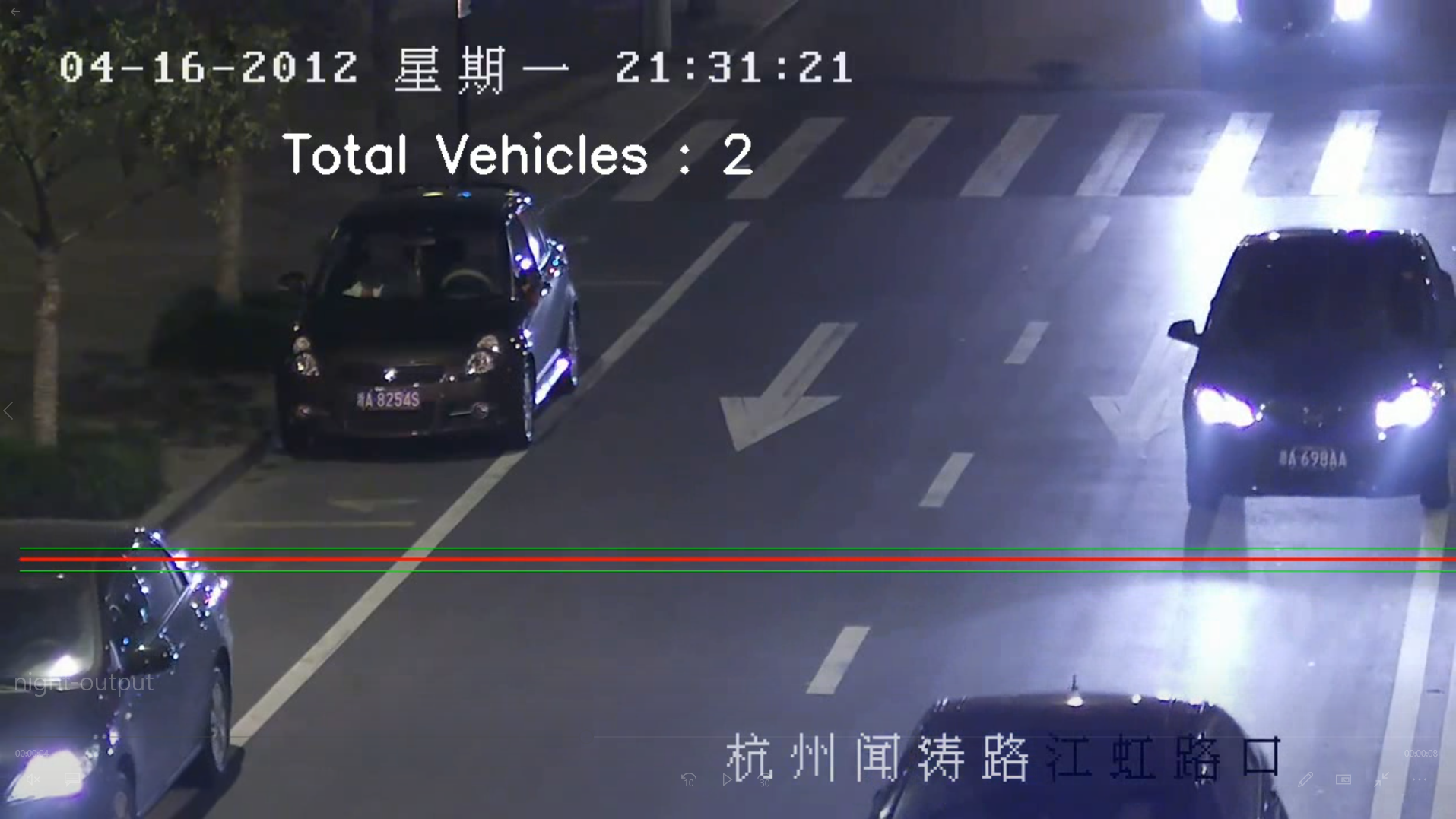
Added Text to display the number of vehicles [Source : GitHub/saakshi077/vehicle-count-model
Endnote
Thank you for reading my first blog 🙂
In this blog, I explained some basic functions of OpenCV Library to get started with learning and using this library.
I am hoping to write some more on the same ( will be in continuation of this blog).
Along with that, I am looking forward to writing the same kind of articles to help you get started with other Computer Vision Libraries.
About the Author
Hey! I am Saakshi Malhotra …
A Computer Science student, passionate about Artificial Intelligence, Deep Learning, and Computer Vision.
I welcome all the suggestions and doubts in the comments section. Thank you for being here : )



%202.jpg)