Basic Statistics Concepts for Machine Learning Newbies!

Introduction

Statistics is a subject that really matters a lot in any technology especially while dealing with data because all the use cases we work on, data is its base, and statistics concepts are required to understand and interpret conclusions from data. Once you can get the basic concepts it will be easy for you to learn and apply Machine Learning concepts. we are going to learn some of the basic and most important statistics topics along with its implementation in python. In this article , you will know about the statistics topics for machine learning, basic statistics for machine learning, so we are covering mostly about the statistics for machine learning.

This article was published as a part of the Data Science Blogathon

For practicals of each statistical term, we will use the Iris dataset which is easily available on Kaggle or you can find it here. And let us be prepared by loading the dataset so it’s easy to apply methods directly.

What is Statistics?

Statistics is the discipline concerned with collecting, organizing, analyzing, interpreting, and presenting data. In simpler terms, it’s the art and science of understanding data.

Basis of Statistics

Statistics is essentially the science of collecting, analyzing, interpreting, presenting, and organizing data. It’s a tool used to make sense of information and draw conclusions.

<div>
<pre>data.rename(columns={'SepalLengthCm':'SL','SepalWidthCm':'SW','PetalLengthCm':'PL','PetalWidthCm':'PW'},inplace=True)
iris_setosa=data[data['Species']=='Iris-setosa']
iris_versicolor=data[data['Species']=='Iris-versicolor']
iris_virginica=data[data['Species']=='Iris-virginica']</pre>
</div>

let’s get started.

Statistics and Its types

Statistics is the discipline that concerns the collection, organization, analysis, interpretation, and presentation of data. There are 2 types of statistics

1) Descriptive statistics

Descriptive statistics is understanding, analyzing, summarizing the data in form of numbers and graphs. We analyze the data using different plots and charts on different kinds of data(numerical and categorical) like bar plot, pie chart, scatter plot, Histogram, etc. All the kind of interpretation, visualizing is part of descriptive statistics. Remember that descriptive statistics can be performed on a sample as well as population data but never do we get or take population data.

2) Inferential statistics

We are extracting some sample of data from population data, and from that sample of data, we are inferencing something(driving conclusion) for population data. It means we perform some tests on sample data and make a conclusion specific to that population. we use various techniques to drive conclusions including data visualization, manipulation, etc.

What is Data in Statistics?

Data in statistics is essentially raw, unprocessed information. It’s the foundation upon which statistical analysis is built. Think of it as the building blocks of knowledge

Types of Data

there are 2 types of data we get as Numerical and Categorical which we need to handle and analyze.

1) Numerical Data –

Numerical data simply means Numbers or integers. Numeric data is further divided into 2 categories and discrete and continuous numerical variables.

I) Discrete Numerical variables – Discrete variables are those whose values are infinite range, for example, rank in the classroom, number of faculties in the department, etc.

II) Continuous Numeric variable – Continuous variables are those whose value can range infinite, means not in the proper range for example salary of an employee.

2) Categorical Data –

Categorical data means categories or programming strings or a character type of data like name and color. generally, these are also of 2 types.

I) Ordinal Variables – Ordinal categorical variable means whose values you can rank between any range like a grade of student(A, B, C), high, medium, and low.

II) Nominal Variables – Nominal variables are variables that cannot be ranked, simply contain names or number of categories like colour name, subjects, etc.

Measure of Central Tendency

A measure of central tendency gives an idea of the centrality of data means what is the centre of your data. It contains various terms like mean, median, and mode.

I) Mean –

mean is only the average of all numbers in a particular numeric variable. when data contains outliers then finding mean and using it in any kind of manipulation is not suggested because a single outlier affects mean badly. so its solution is median.

# find mean each class Sepal Width
print(np.mean(iris_setosa['SW']))
print(np.mean(iris_versicolor['SW']))
print(np.mean(iris_virginica['SW']))

II) Median –

the median is a centre value after sorting all the numbers. if the total number is even then it is the average of centre 2 values. It does not depend on or affected outliers till half of the data does not become outliers.

# find median of each class Petal Length
print(np.median(iris_setosa['PL']))
print(np.median(iris_versicolor['PL']))
print(np.median(iris_virginica['PL']))

III) Mode –

Mode represents the most frequent observation in a numeric variable. To find mode we do not have a function in Numpy, but we have a function in scipy.

#find mode of petal length of each class
from scipy import stats
print(stats.mode(iris_setosa['PL']))
print(stats.mode(iris_versicolor['PL']))
print(stats.mode(iris_virginica['PL']))

Never use one of these three things, try to use all three so that you can understand the nature of data.

Measures of Spread

Measures of spread help to understand spreads of data means where your data is more spread (positive, negative, center)

I) Range –

The range describes the difference between the largest and smallest point in your data (max-min).

#find range of setosa petal length flower leaves
r=np.max(iris_setosa['PL']) - np.min(iris_setosa['PL'])
print("The range is",r)

II) Percentiles –

A percentile is a measure used in statistics indicating the value below which a given percentage of observation in a group of observations falls. for example, the 20th percentile is a value below which 20 per cent of data falls. we use percentile much in a real-world scenario like in JEE Mains exam. Or you can say like 20 percentile is 35 so we can say that total 20percentile observation having a value less than 1.

mylist=[1,2,3,4,5,6,7,8,9]
print(np.percentile(mylist,25))
print(np.percentile(mylist,90))
#find setosa flowers 95th percentile value
np.percentile(iris_setosa['PL'],95)

III) Quartiles –

Quartiles are the values that divide a list of numbers into quarters. the steps to find the quartile is.

• Put the list of numbers in order
• Then cut the list into 4 equal parts
• The quartiles are at the cuts

Q2 is also known as the median and we can find the 4 quartiles by depicting the percentile value at 25, 50, 75, and 100.

print(np.percentile(iris_setosa['PL'],25))
print(np.percentile(iris_setosa['PL'],50))
print(np.percentile(iris_setosa['PL'],75))
print(np.percentile(iris_setosa['PL'],100))

IV) Interquartile Range(IQR) – It is a measure of dispersion between upper(75th) and lower(25th) Quartiles. It is a very important term in statistics that is used in most calculations and data preprocessing like dealing with outliers.

V) Mean Absolute Deviation –

The absolute deviation from the mean, also called Mean absolute deviation(MAD), describes the variation in the data set. In simple words, it tells the average absolute distance of each point in the set.

MAD = ∑∣xi​−xˉ∣​ / n

Eg- set of numbers = [2, 5, 1, 6, , 7, 3, 11]
the mean is 5
find difference - |2-5| + |5-5| + |1-5| + |6-5| + |7-5| + |3-5| + |11-5|
3+0+4+1+2+2+6 = 18/7 = 2.5

VI) Variance –

Variance measure how far is data point is from the mean, only the difference from MAD and variance is we take square here. The variance is computed by finding the difference between each data point and mean, squaring them, summing them up, and take the average of all those numbers. the numpy has a direct function to calculate variance.

np.var(iris_setosa['PL'])

The problem with variance

The problem with variance is that because of a square, it is not in the same unit of measurement as of original data. So, it’s not too intuitive to use it so people mostly preferred standard deviation.

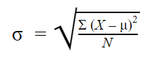
VII) Standard Deviation –

As we saw due to squaring the original unit changes so, the standard deviation is simply the square root of variance so we get again the value in the same measurement. And we can directly calculate the standard deviation using Numpy.

np.std(iris_setosa['PL'])

VIII) Median Absolute Deviation – MAD is the median of all the numbers obtained from subtracting and calculating the absolute value of every observation with the median. numpy does not have a function for MAD but stats models have a package called robust which contains MAD function.

from statsmodels import robust
mad = robust.mad(np.array([1,3,5,6,7,8,9]))
print(mad)

Normal Distribution in statistics

A normal distribution is a distribution in form of a bell curve and most of the datasets in machine learning follow a normal distribution and if not then we try to transform it into normal distribution and many machine learning algorithms work very well on this distribution because in real-world scenario also many use cases follow this distribution like salary, very fewer employees will be there that are having less salary, and very less employee with very high salary and most of the employees will lie in middle or in the medium range.

If any data follows Normal or Gaussian distribution then it also follows three conditions known as Empirical Formula

• P[ mean – std_dev <= mean + std_dev] = 68 percent
• P[ mean – 2* std_dev <= mean + 2*std_dev] = 95 percent
• P[ mean – 3*std_dev <= mean + 3*std_dev] = 99.7 percent

You analyze this things while performing exploratory data analysis. We can also convert any variable distribution into Standard Normal Distribution.

Skewness

Skewness is a measure of the symmetry of distribution that you plot in form of a histogram, KDE which has a high peak towards the mode of data. skewness is generally of 2 types as left-skewed data and right-skewed data. Some also understand as 3 types where third is symmetric distribution means Normal distribution.

I) Right Skewed Data(Positively skewed distribution)

Right skewed distribution means data that has a long tail towards the right side(Positive axis). A classical example of right-skewed is wealth distribution, there are very less few people who have very high wealth and maximum people are in the medium range. I would encourage you to mention more examples in the comment box.

II) Left-skewed Data(Negatively skewed distribution)

Left skewed distribution means data that has a long tail towards the left side(negative axis). An example can be Grades of students, there will be fewer students who have received fewer grades and the maximum student will be in the pass category.

Central Limit Theorem

Central Limit Theorem states that, when we analyze the sample data of any population then after doing some statistical measure, If you see that mean of standard deviation and sample mean will be approximately the same. This is only the central Limit theorem.

Probability Density Function(PDF)

If you know about Histogram then where you cut the data in bins, and visualize spread. But if we want to do a multiclass sort of analysis on numerical data, then it is difficult to do using Histogram and It can be easily be done using PDF. The probability density function is that line drawn within histogram only using KDE(kernel density estimation). So, if you see the KDE curve it passes by touching the corner of each bin. Hence using PDF we can draw side by side KDE and analysis multiclass data.

<div>
<pre>sns.FacetGrid(data, hue='Species', height=6).map(sns.distplot, 'PL').add_legend()
plt.show()</pre>
</div>

In the above plot if I ask that, I want to write 3 conditions that distinguish classify 3 classes then how can I do that? Let us do this using histogram and PDF and understand the comparison between both.

<div>
<pre>sns.FacetGrid(data, hue='Species', height=6).map(sns.distplot, 'PL', kde=False).add_legend()
plt.show()</pre>
</div>

From the above histogram, we can write that if a value is less than 2 then It is setosa. If greater than 2 and less than 4.5 then it’s Versicolor, then up to the certain point we are right but after 4.5 also there is Versicolor and from 5 to 7 it’s Virginica. the overlap area will disturb you, and here PDF is going to help you out.

Now PDF will help you to write some smart cases. Condition for setosa is the same as less than 2. For another 2 classes, we can take the intersecting point of both the curve then chances for correct classification will increase compared to a histogram.

Cumulative Distributive function(CDF)

CDF tells us that how much percentage of data is less than a particular number. To find the CDF we will add all the histogram bind before that point and the result will be my resultant CDF. Another method to do so is using Calculus using Area under the curve, so at what point you want CDF, plot the straight line from that and find the inner area. Hence on integrating PDF we get CDF and on differentiating CDF we get PDF.

How to calculate PDF and CDF

we will calculate the PDF and CDF for setosa. we convert the petal length into 10 bins and extract out the frequency count of each bin and the edges of each which give the point where the bin starts and where it ends. To calculate PDF we divide each frequency count value with the total sum and we get the probability density function and if we find the cumulative sum of PDF we get CDF.

<div>
<pre>counts, bin_edges = np.histogram(iris_setosa['PL'], bins=10)
pdf = counts / sum(counts)
cdf = np.cumsum(pdf)
print(pdf)
print(cdf)</pre>
</div>

Conclusion

We have learned about statistics and its importance in Machine learning. We started with types of statistics, what are types of data we deal with, and we have seen basic terms we require to perform some mathematical and statistical operation to understand the nature of data. Some more topics like covariance, hypothesis testing, Chebyshev inequality, etc which we will study in the next part of this article.

Hope you like the article and now get understanding about the basic statistics concepts, statistics for machine learning and various statistics topics for machine learning.

I hope it was easy to catch up on this topic, If you have any queries, please post them in the comment section below. If you like the article, give a read to my other articles also. link

Raghav Agrawal

I am a software Engineer with a keen passion towards data science. I love to learn and explore different data-related techniques and technologies. Writing articles provide me with the skill of research and the ability to make others understand what I learned. I aspire to grow as a prominent data architect through my profession and technical content writing as a passion.