1. Objective
In this article, we will be predicting the prices of used cars. We will be building various Machine Learning models and Deep Learning models with different architectures. In the end, we will see how machine learning models perform in comparison to deep learning models.
2. Data Used
Here we have used the data from a hiring competition that was live on machinehack.com Use the below link to access the data and use it for your analysis.
MATHCO.THON: The Data Scientist Hiring Hackathon by TheMathCompany (machinehack.com)
3. Data Inspection
In this section, we will explore the data. First Let’s see what columns we have in the data and their data types along with missing values information.
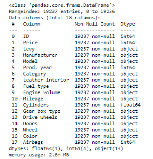
We can observe that data have 19237 rows and 18 columns.
There are 5 numeric columns and 13 categorical columns. With the first look, we can see that there are no missing values in the data.
‘Price‘ column/feature is going to be the target column or dependent feature for this project.
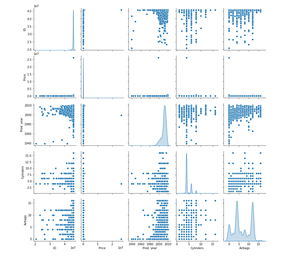
Let’s see the distribution of the data.
4. Data Preparation
Here we will clean the data and prepare it for training the model.
‘ID’ column
We are dropping the ‘ID’ column since it does not hold any significance for car Price prediction.
df.drop('ID',axis=1,inplace=True)
‘Levy’ column
After analyzing the ‘Levy’ column we found out that it does contain the missing values but it was given as ‘-‘ in the data and that’s why we were not able to capture the missing values earlier in the data.
Here we will impute ‘-‘ in the ‘Levy’ column with ‘0’ assuming there was no ‘Levy’. We can also impute it with ‘mean’ or ‘median’, but that’s a choice that you have to make.
df['Levy']=df['Levy'].replace('-',np.nan)
df['Levy']=df['Levy'].astype(float)
levy_mean=0
df['Levy'].fillna(levy_mean,inplace=True)
df['Levy']=round(df['Levy'],2)
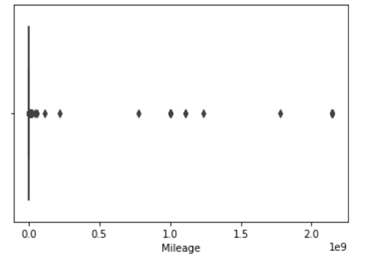
‘Mileage’ column
‘Mileage’ column here means how many kilometres the car has driven. ‘km’ is written in the column after each reading. We will remove that.
#since milage is in KM only we will remove 'km' from it and make it numerical
df['Mileage']=df['Mileage'].apply(lambda x:x.split(' ')[0])
df['Mileage']=df['Mileage'].astype('int')
‘Engine Volume’ column
In the ‘Engine Volumn’ column along with the Engine Volumn ‘type’ of the engine(Turbo or not Turbo) is also written. We will create a new column that shows the ‘type’ of ‘Engine’.
df['Turbo']=df['Engine volume'].apply(lambda x:1 if 'Turbo' in str(x) else 0)
df['Engine volume']=df['Engine volume'].apply(lambda x:str(x).replace('Turbo',''))
df['Engine volume']=df['Engine volume'].astype(float)
‘Doors’ Column
df['Doors'].unique()
Output:
‘Doors’ column represents the number of doors in the car. But as we can see it is not clean. Let’s clean
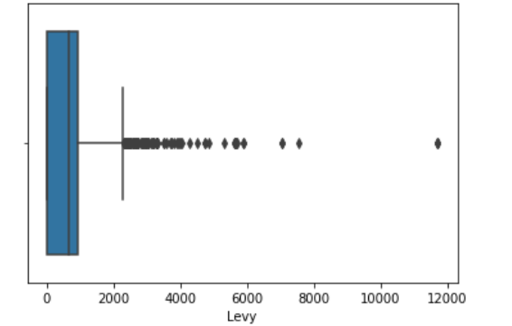
Handling ‘Outliers’
This we will examine across numerical features.
cols=['Levy','Engine volume', 'Mileage','Cylinders','Airbags']
sns.boxplot(df[cols[0]]);
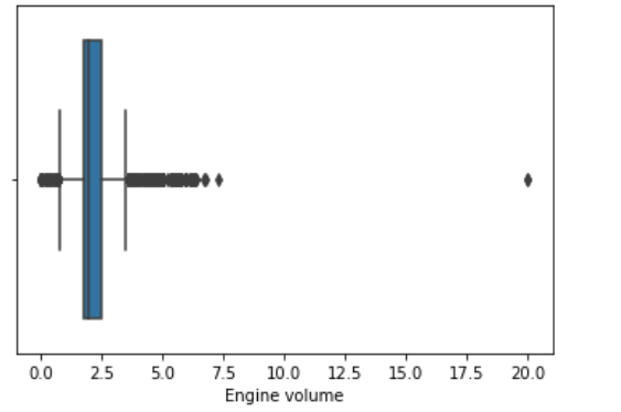
sns.boxplot(df[cols[1]]);
sns.boxplot(df[cols[2]]);
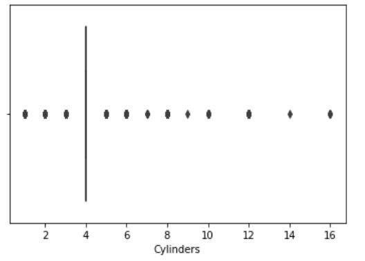
sns.boxplot(df[cols[3]]);
sns.boxplot(df[cols[4]]);
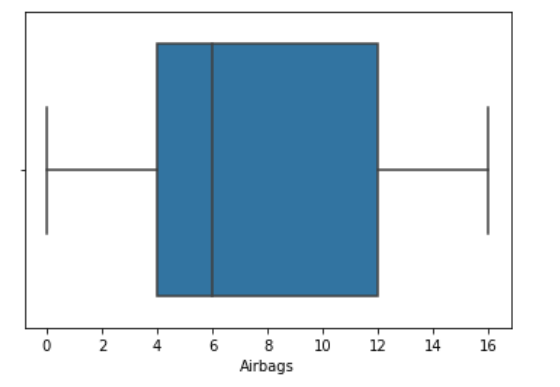
As we can see there are outliers in ‘Levy’,’Engine volume’, ‘Mileage’, ‘Cylinders’ columns. We will remove these outliers using Inter Quantile Range(IQR) method.
def find_outliers_limit(df,col):
    print(col)
    print('-'*50)
    #removing outliers
    q25, q75 = np.percentile(df[col], 25), np.percentile(df[col], 75)
    iqr = q75 - q25
    print('Percentiles: 25th=%.3f, 75th=%.3f, IQR=%.3f' % (q25, q75, iqr))
    # calculate the outlier cutoff
    cut_off = iqr * 1.5
    lower, upper = q25 - cut_off, q75 + cut_off
    print('Lower:',lower,' Upper:',upper)
    return lower,upper
def remove_outlier(df,col,upper,lower):
    # identify outliers
    outliers = [x for x in df[col] if x  upper]
    print('Identified outliers: %d' % len(outliers))
    # remove outliers
    outliers_removed = [x for x in df[col] if x >= lower and x <= upper]
    print('Non-outlier observations: %d' % len(outliers_removed))
    final= np.where(df[col]>upper,upper,np.where(df[col]<lower,lower,df[col]))
    return final
outlier_cols=['Levy','Engine volume','Mileage','Cylinders']
for col in outlier_cols:
    lower,upper=find_outliers_limit(df,col)
    df[col]=remove_outlier(df,col,upper,lower)
Let’s examine the features after removing outliers.
plt.figure(figsize=(20,10))
df[outlier_cols].boxplot()
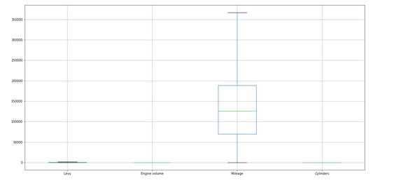
We can observe that there are no outliers in the features now.
Creating Additional Features
We see that ‘Mileage’ and ‘Engine Volume’ are continuous variables. While performing regression I have observed that binning such variables can help increase the performance of the model. So I am creating the ‘Bin’ features for these features/columns.
labels=[0,1,2,3,4,5,6,7,8,9]
df['Mileage_bin']=pd.cut(df['Mileage'],len(labels),labels=labels)
df['Mileage_bin']=df['Mileage_bin'].astype(float)
labels=[0,1,2,3,4]
df['EV_bin']=pd.cut(df['Engine volume'],len(labels),labels=labels)
df['EV_bin']=df['EV_bin'].astype(float)
Handling Categorical features
I have used Ordinal Encoder to handle the categorical columns. OrdinalEncoder works similar to LabelEncoder but OrdinalEncoder can be applied to multiple features while LabelEncoder can be applied to One feature at a time. For more details please visit the below links
LabelEncoder:https://scikit-learn.org/stable/modules/generated/sklearn.preprocessing.LabelEncoder.html
OrdinalEncoder:https://scikit-learn.org/stable/modules/generated/sklearn.preprocessing.OrdinalEncoder.html
num_df=df.select_dtypes(include=np.number)

cat_df=df.select_dtypes(include=object)

encoding=OrdinalEncoder()

cat_cols=cat_df.columns.tolist()

encoding.fit(cat_df[cat_cols])

cat_oe=encoding.transform(cat_df[cat_cols])

cat_oe=pd.DataFrame(cat_oe,columns=cat_cols)

cat_df.reset_index(inplace=True,drop=True)

cat_oe.head()

num_df.reset_index(inplace=True,drop=True)

cat_oe.reset_index(inplace=True,drop=True)

final_all_df=pd.concat([num_df,cat_oe],axis=1)
Checking correlation
final_all_df['price_log']=np.log(final_all_df['Price'])
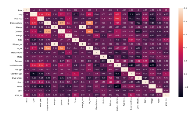
We can observe that features are not much correlated in the data. But there is one thing that we can notice is that after log transforming ‘Price’ column, correlation with few features got increased which is a good thing. We will be using log-transformed ‘Price’ to train the model. Please visit mentioned link below to better understand how feature transformations help improve model performance.
https://www.analyticsvidhya.com/blog/2020/07/types-of-feature-transformation-and-scaling/
5. Data Splitting and Scaling
We have done an 80-20 split on the data. 80% of the data will be used for training and 20% data will be used for testing.
We will also scale the data since feature values in data do not have the same scale and having different scales can produce poor model performance.
cols_drop=['Price','price_log','Cylinders']
X=final_all_df.drop(cols_drop,axis=1)
y=final_all_df['Price']
X_train,X_test,y_train,y_test=train_test_split(X,y,test_size=0.2,random_state=25)
scaler=StandardScaler()
X_train_scaled=scaler.fit_transform(X_train)
X_test_scaled=scaler.transform(X_test)
6. Model Building
We built LinearRegression, XGBoost, and RandomForest as machine learning models and two deep learning models one having a small network and another having a large network.
We built base models of LinearRegression, XGBoost, and RandomForest so there is not much to show about these models but we can see the model summary and how they converge with deep learning models that we built.
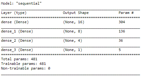
Deep Learning Model – Small Network model summary
model_dl_small.summary()
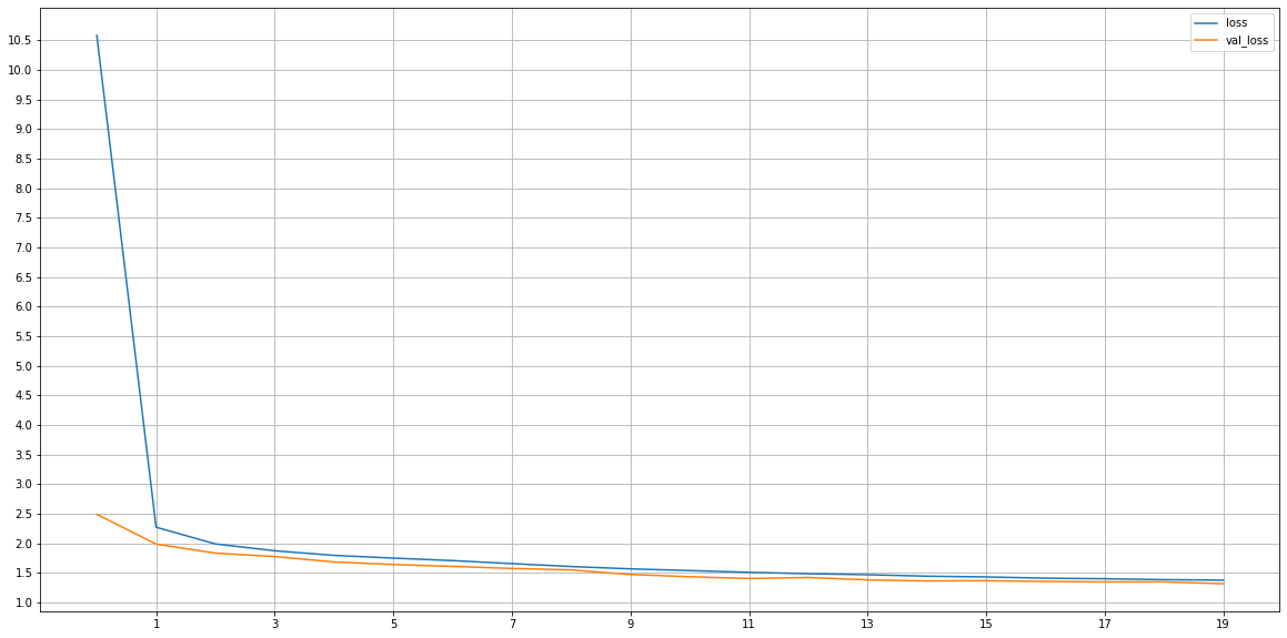
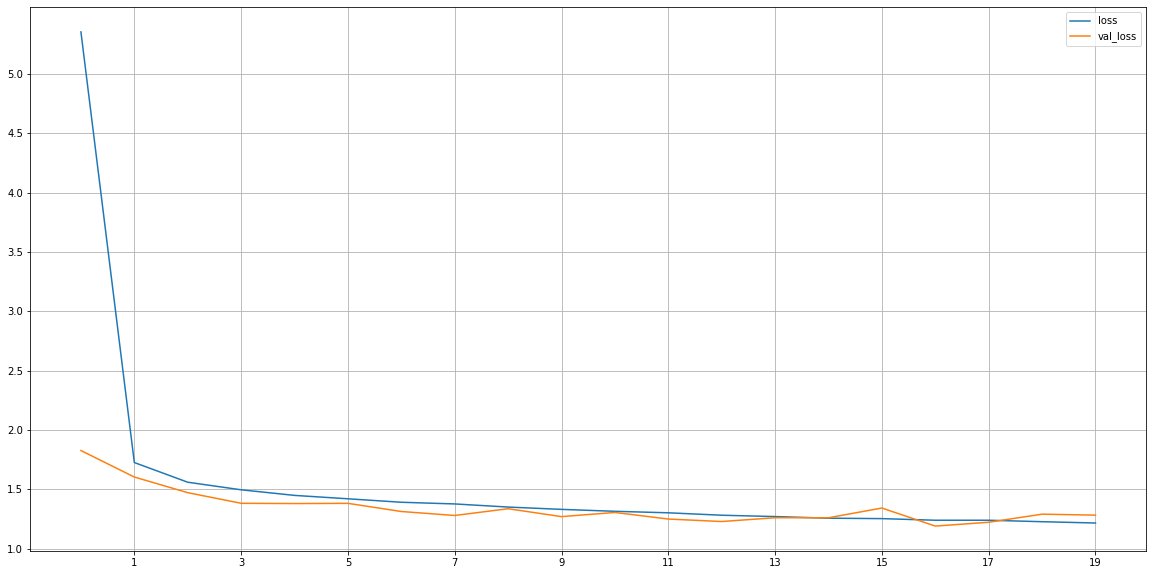
Deep Learning Model – Small Network _Train & Validation Loss
#plot the loss and validation loss of the dataset
history_df = pd.DataFrame(model_dl_small.history.history)
plt.figure(figsize=(20,10))
plt.plot(history_df['loss'], label='loss')
plt.plot(history_df['val_loss'], label='val_loss')
plt.xticks(np.arange(1,epochs+1,2))
plt.yticks(np.arange(1,max(history_df['loss']),0.5))
plt.legend()
plt.grid()
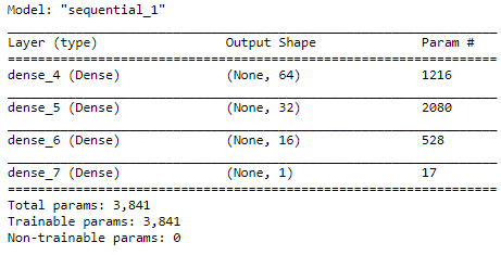
Deep Learning Model – Large Network model summary
model_dl_large.summary()
Deep Learning Model – Large Network _Train & Validation Loss
#plot the loss and validation loss of the dataset
history_df = pd.DataFrame(model_dl_large.history.history)
plt.figure(figsize=(20,10))
plt.plot(history_df['loss'], label='loss')
plt.plot(history_df['val_loss'], label='val_loss')
plt.xticks(np.arange(1,epochs+1,2))
plt.yticks(np.arange(1,max(history_df['loss']),0.5))
plt.legend()
plt.grid()
6.1 Model Performance
We have evaluated the models using Mean_Squared_Error, Mean_Absolute_Error, Mean_Absolute_Percentage_Error, Mean_Squared_Log_Error as performance matrices, and below are the results we got.
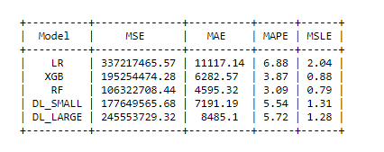
We can observe that Deep Learning Model did not perform well in comparison with Machine Learning Models. RandomForest performed really well among Machine Learning Model.
Let’s visualize the results from Random Forest.
7. Result Visualization
y_pred=np.exp(model_rf.predict(X_test_scaled))
number_of_observations=20
x_ax = range(len(y_test[:number_of_observations]))
plt.figure(figsize=(20,10))
plt.plot(x_ax, y_test[:number_of_observations], label="True")
plt.plot(x_ax, y_pred[:number_of_observations], label="Predicted")
plt.title("Car Price - True vs Predicted data")
plt.xlabel('Observation Number')
plt.ylabel('Price')
plt.xticks(np.arange(number_of_observations))
plt.legend()
plt.grid()
plt.show()
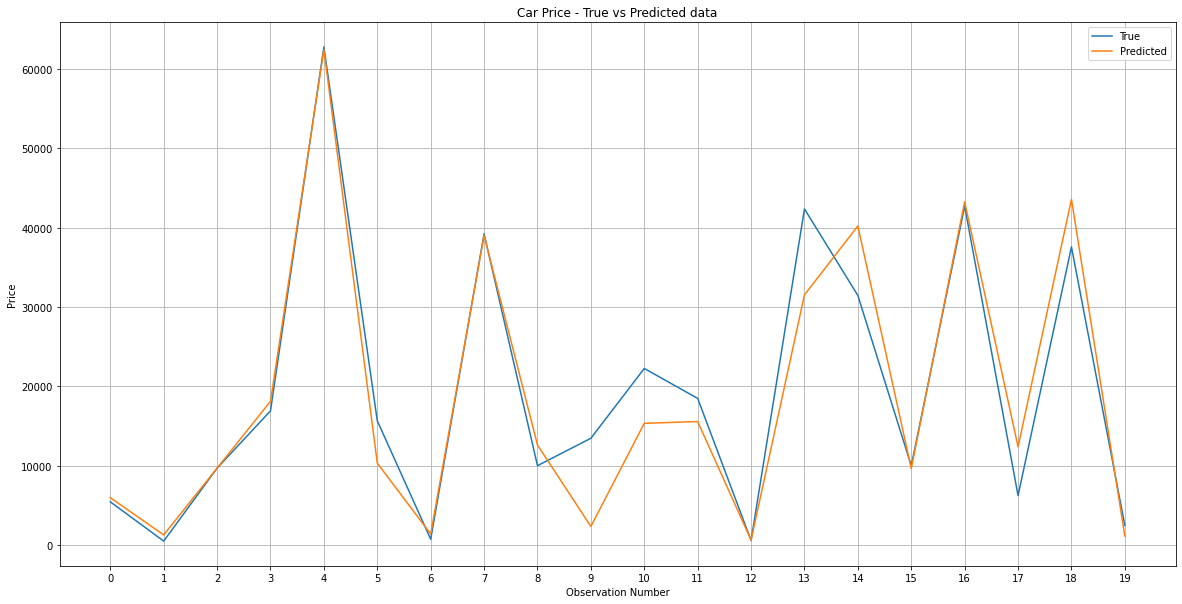
We can observe in the graph that the model is performing really well as seen in performance matrices as well.
8. Code
Code was done on jupyter notebook. Below is the complete code for the project.
# Loading Libraries

import pandas as pd

import numpy as np

from sklearn.preprocessing import OrdinalEncoder

from sklearn.model_selection import train_test_split

from sklearn.metrics import mean_squared_log_error,mean_squared_error,mean_absolute_error,mean_absolute_percentage_error

import datetime

from sklearn.ensemble import RandomForestRegressor

from sklearn.linear_model import LinearRegression

from xgboost import XGBRegressor

from sklearn.preprocessing import StandardScaler

import matplotlib.pyplot as plt

import seaborn as sns

from keras.models import Sequential

from keras.layers import Dense

from prettytable import PrettyTable

df=pd.read_csv('../input/Participant_Data_TheMathCompany_.DSHH/train.csv')

df.head()

# Data Inspection

df.shape

df.describe().transpose()

df.info()

sns.pairplot(df, diag_kind='kde')

# Data Preprocessing

df.drop('ID',axis=1,inplace=True)

df['Levy']=df['Levy'].replace('-',np.nan)

df['Levy']=df['Levy'].astype(float)

levy_mean=0

df['Levy'].fillna(levy_mean,inplace=True)

df['Levy']=round(df['Levy'],2)

milage_formats=set()

def get_milage_format(x):

    x=x.split(' ')[1]

    milage_formats.add(x)

df['Mileage'].apply(lambda x:get_milage_format(x));

milage_formats

#since milage is in KM only we will remove 'km' from it and make it numerical

df['Mileage']=df['Mileage'].apply(lambda x:x.split(' ')[0])

df['Mileage']=df['Mileage'].astype('int')

df['Engine volume'].unique()

df['Turbo']=df['Engine volume'].apply(lambda x:1 if 'Turbo' in str(x) else 0)

df['Engine volume']=df['Engine volume'].apply(lambda x:str(x).replace('Turbo',''))

df['Engine volume']=df['Engine volume'].astype(float)

cols=['Levy','Engine volume', 'Mileage','Cylinders','Airbags']

sns.boxplot(df[cols[0]]);

cols=['Levy','Engine volume', 'Mileage','Cylinders','Airbags']

sns.boxplot(df[cols[1]]);

cols=['Levy','Engine volume', 'Mileage','Cylinders','Airbags']

sns.boxplot(df[cols[2]]);

cols=['Levy','Engine volume', 'Mileage','Cylinders','Airbags']

sns.boxplot(df[cols[3]]);

cols=['Levy','Engine volume', 'Mileage','Cylinders','Airbags']

sns.boxplot(df[cols[4]]);

def find_outliers_limit(df,col):

    print(col)

    print('-'*50)

    #removing outliers

    q25, q75 = np.percentile(df[col], 25), np.percentile(df[col], 75)

    iqr = q75 - q25

    print('Percentiles: 25th=%.3f, 75th=%.3f, IQR=%.3f' % (q25, q75, iqr))

    # calculate the outlier cutoff

    cut_off = iqr * 1.5

    lower, upper = q25 - cut_off, q75 + cut_off

    print('Lower:',lower,' Upper:',upper)

    return lower,upper

def remove_outlier(df,col,upper,lower):

    # identify outliers

    outliers = [x for x in df[col] if x  upper]

    print('Identified outliers: %d' % len(outliers))

    # remove outliers

    outliers_removed = [x for x in df[col] if x >= lower and x <= upper]

    print('Non-outlier observations: %d' % len(outliers_removed))

    final= np.where(df[col]>upper,upper,np.where(df[col]<lower,lower,df[col]))

    return final

outlier_cols=['Levy','Engine volume','Mileage','Cylinders']

for col in outlier_cols:

    lower,upper=find_outliers_limit(df,col)

    df[col]=remove_outlier(df,col,upper,lower)

#boxplot - to see outliers

plt.figure(figsize=(20,10))

df[outlier_cols].boxplot()

df['Doors'].unique()

df['Doors']=df['Doors'].map({'04-May':'4_5','02-Mar':'2_3','>5':'5'})

df['Doors']=df['Doors'].astype(str)

#Creating Additional Features

labels=[0,1,2,3,4,5,6,7,8,9]

df['Mileage_bin']=pd.cut(df['Mileage'],len(labels),labels=labels)

df['Mileage_bin']=df['Mileage_bin'].astype(float)

labels=[0,1,2,3,4]

df['EV_bin']=pd.cut(df['Engine volume'],len(labels),labels=labels)

df['EV_bin']=df['EV_bin'].astype(float)

#Handling Categorical features

num_df=df.select_dtypes(include=np.number)

cat_df=df.select_dtypes(include=object)

encoding=OrdinalEncoder()

cat_cols=cat_df.columns.tolist()

encoding.fit(cat_df[cat_cols])

cat_oe=encoding.transform(cat_df[cat_cols])

cat_oe=pd.DataFrame(cat_oe,columns=cat_cols)

cat_df.reset_index(inplace=True,drop=True)

cat_oe.head()

num_df.reset_index(inplace=True,drop=True)

cat_oe.reset_index(inplace=True,drop=True)

final_all_df=pd.concat([num_df,cat_oe],axis=1)

#Checking correlation

final_all_df['price_log']=np.log(final_all_df['Price'])

plt.figure(figsize=(20,10))

sns.heatmap(round(final_all_df.corr(),2),annot=True);

cols_drop=['Price','price_log','Cylinders']

final_all_df.columns

X=final_all_df.drop(cols_drop,axis=1)

y=final_all_df['Price']

# Data Splitting and Scaling

X_train,X_test,y_train,y_test=train_test_split(X,y,test_size=0.2,random_state=25)

scaler=StandardScaler()

X_train_scaled=scaler.fit_transform(X_train)

X_test_scaled=scaler.transform(X_test)

# Model Building

def train_ml_model(x,y,model_type):

    if model_type=='lr':

        model=LinearRegression()

    elif model_type=='xgb':

        model=XGBRegressor()

    elif model_type=='rf':

        model=RandomForestRegressor()

    model.fit(X_train_scaled,np.log(y))

    return model

def model_evaluate(model,x,y):

    predictions=model.predict(x)

    predictions=np.exp(predictions)

    mse=mean_squared_error(y,predictions)

    mae=mean_absolute_error(y,predictions)

    mape=mean_absolute_percentage_error(y,predictions)

    msle=mean_squared_log_error(y,predictions)

    mse=round(mse,2)

    mae=round(mae,2)

    mape=round(mape,2)

    msle=round(msle,2)

    return [mse,mae,mape,msle]

model_lr=train_ml_model(X_train_scaled,y_train,'lr')

model_xgb=train_ml_model(X_train_scaled,y_train,'xgb')

model_rf=train_ml_model(X_train_scaled,y_train,'rf')

## Deep Learning

### Small Network

model_dl_small=Sequential()

model_dl_small.add(Dense(16,input_dim=X_train_scaled.shape[1],activation='relu'))

model_dl_small.add(Dense(8,activation='relu'))

model_dl_small.add(Dense(4,activation='relu'))

model_dl_small.add(Dense(1,activation='linear'))

model_dl_small.compile(loss='mean_squared_error',optimizer='adam')

model_dl_small.summary()

epochs=20

batch_size=10

model_dl_small.fit(X_train_scaled,np.log(y_train),verbose=0,validation_data=(X_test_scaled,np.log(y_test)),epochs=epochs,batch_size=batch_size)

#plot the loss and validation loss of the dataset

history_df = pd.DataFrame(model_dl_small.history.history)

plt.figure(figsize=(20,10))

plt.plot(history_df['loss'], label='loss')

plt.plot(history_df['val_loss'], label='val_loss')

plt.xticks(np.arange(1,epochs+1,2))

plt.yticks(np.arange(1,max(history_df['loss']),0.5))

plt.legend()

plt.grid()

### Large Network

model_dl_large=Sequential()

model_dl_large.add(Dense(64,input_dim=X_train_scaled.shape[1],activation='relu'))

model_dl_large.add(Dense(32,activation='relu'))

model_dl_large.add(Dense(16,activation='relu'))

model_dl_large.add(Dense(1,activation='linear'))

model_dl_large.compile(loss='mean_squared_error',optimizer='adam')

model_dl_large.summary()

epochs=20

batch_size=10

model_dl_large.fit(X_train_scaled,np.log(y_train),verbose=0,validation_data=(X_test_scaled,np.log(y_test)),epochs=epochs,batch_size=batch_size)

#plot the loss and validation loss of the dataset

history_df = pd.DataFrame(model_dl_large.history.history)

plt.figure(figsize=(20,10))

plt.plot(history_df['loss'], label='loss')

plt.plot(history_df['val_loss'], label='val_loss')

plt.xticks(np.arange(1,epochs+1,2))

plt.yticks(np.arange(1,max(history_df['loss']),0.5))

plt.legend()

plt.grid()

summary=PrettyTable(['Model','MSE','MAE','MAPE','MSLE'])

summary.add_row(['LR']+model_evaluate(model_lr,X_test_scaled,y_test))

summary.add_row(['XGB']+model_evaluate(model_xgb,X_test_scaled,y_test))

summary.add_row(['RF']+model_evaluate(model_rf,X_test_scaled,y_test))

summary.add_row(['DL_SMALL']+model_evaluate(model_dl_small,X_test_scaled,y_test))

summary.add_row(['DL_LARGE']+model_evaluate(model_dl_large,X_test_scaled,y_test))

print(summary)

y_pred=np.exp(model_rf.predict(X_test_scaled))

number_of_observations=20

x_ax = range(len(y_test[:number_of_observations]))

plt.figure(figsize=(20,10))

plt.plot(x_ax, y_test[:number_of_observations], label="True")

plt.plot(x_ax, y_pred[:number_of_observations], label="Predicted")

plt.title("Car Price - True vs Predicted data")

plt.xlabel('Observation Number')

plt.ylabel('Price')

plt.xticks(np.arange(number_of_observations))

plt.legend()

plt.grid()

plt.show()
9.Conclusion
In this article, we tried predicting the car price using the various parameters that were provided in the data about the car. We build machine learning and deep learning models to predict car prices and saw that machine learning-based models performed well at this data than deep learning-based models.
10. About the Author
Hi, I am Kajal Kumari. I have completed my Master’s from IIT(ISM) Dhanbad in Computer Science & Engineering. As of now, I am working as Machine Learning Engineer in Hyderabad. You can also check out few other blogs that I have written here.
The media shown in this article on LSTM for Human Activity Recognition are not owned by Analytics Vidhya and are used at the Author’s discretion.
Hi, I am Kajal Kumari. have completed my Master’s from IIT(ISM) Dhanbad in Computer Science & Engineering. As of now, I am working as Machine Learning Engineer in Hyderabad.
hope that you have enjoyed the article. If you like it, share it with your friends also. Please feel free to comment if you have any thoughts that can improve my article writing.
If you want to read my previous blogs, you can read Previous Data Science Blog posts here. Connect with me


Hi that is a normal behavior. Deep learning is made for unstructured data ( image, sounds, etc). It works poorly on structured data like the one presented here, compared to RF.
Hi, I have a few doubts, if you could help with this would be very helpful. You have used ordinal encoding directly for all categorical, i thot we should only use ordinal encoding when there is some sort of hierarchical order in the categories like that of education and such. Here we have manufacturer and model so things like these needs to be one hot encoded right ? Also i was getting the negative values for the regression for this. what should we do at this point is it ok to impute these as 0 or should i retrain the model so that i dont get negative values because i read somewhere that negative predictions tend to happen for regression