This article was published as a part of the Data Science Blogathon.
In this article, we discuss how to cook the data for your machine learning algorithms. So that when you feed it, our algorithm will grow taller and stronger 🙂
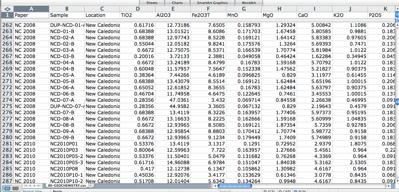
Technically, today we will learn how to prepare our data for Machine Learning Algorithms. In the world of Machine Learning, we call this data pre-processing and also implement them practically. We will be using the Housing Dataset for understanding the concepts.

Introduction:
Firstly, let’s take things a little bit slow, and see what do we mean by data-preprocessing? and why do we need it in the first place? following that we will see methods that will help us in getting tasty data (pre-processed) which will make our machine learning algorithm stronger (accurate).
Table of content:
- What do we mean by data pre-processing and why do we need it.
- Data Cleaning.
- Text and Categorical attributes.
- Feature Scaling.
- Transformation pipelines.
1. What do we mean by data pre-processing and why do we need it?
So what is the first thing that comes up to your mind when you think about data, you might be thinking this:
large datasets with lots of rows and columns. That is a likely scenario, but that may not be the case always.
Data could be in so many different types of forms like audios, videos, images, etc. The machine still doesn’t understand this type of data yet! They are still dumb! all they know is 1s and 0s.
In the world of machine learning, Data pre-processing is basically a step in which we transform, encode, or bring the data to such a state that our algorithm can understand easily.
Let’s go ahead and cook (prepare) the data!!
Instead of doing this manually, always keep a habit of making functions for this purpose, for several good reasons:
- If you are working on a new dataset, and already have functions pre-build reproducing your transformation would be a piece of cake for you.
- Gradually you will be building a library of these functions for your upcoming projects.
- Also, you can directly use these functions in your live project to transform your new data before feeding it to your algorithm.
- You can easily try your various transformation and see which combinations work out best for you.
So without further ado, Let’s get started!
2. Data Cleaning:

The first and foremost step in preparing the data is you need to clean your data. There are a lot of machine learning algorithms(almost all) that cannot work with missing features.
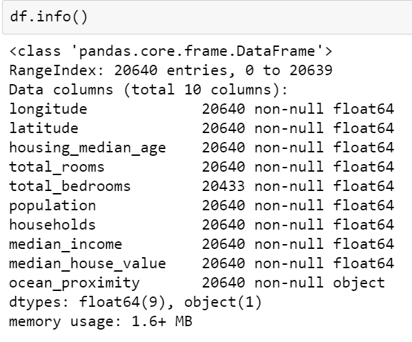
As we can see that there are a couple of missing values in total_bedrooms. Let’s go ahead and create some functions to take care of them.
Now you have three options here:
Remove all the Null values.
df.dropna(subset=["total_bedrooms"])
Remove the entire attribute.
df.drop("total_bedrooms",axis=1)
Replace missing values with some other values(mean, median, or 0).
median = df['total_bedrooms'].median()
df['totalbedrooms'].fillna(mediun, inplace=True)
Most of us go with replacing missing values with median values. Always remember to save the median values that you have calculated, you will be needing it, later on, to replace missing values in the test set and also when your project is live.
So there is an amazing class available in Scikit-Learn which helps us in taking care of missing values.
Simple Imputer !!
Let me show you how to use it,
Create an instance and specify your strategy i.e. median.
from sklearn.impute import SimpleImputer
imputer  = SimpleImputer(strategy="median")
imputer_df = df.drop("ocean_proximity",axis=1)
As we know that, ocean_proximity is text and we cannot compute its median. Hence, we need to remove it at the time of calculations.
Now we can fit the imputer instances that we created onto our training data using the fit() method:
imputer.fit(imputer_df)

Here all the values are set by default;
The imputer we created has calculated the median for all the attributes and stored it in the statistics_ variable. In our case, total_bedrooms was the only one with missing values, but in the future, we can get missing values in other attributes too, So it is good to apply imputer to all attributes to be on a safer side.
imputer.statistics_

Now we will transform our dataset, doing so will return a NumPy array which we will be converting back to the pandas data frame.
X = imputer.transform(imputer_df)
revised_df = pd.DataFrame(X,columns=imputer_df.columns,index = imputer_df.index)
revised_df.info()
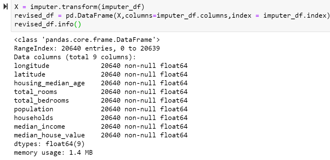
As we can see, all the Null values are now replaced with their corresponding medians.
3. Text and categorical attributes:

A Proper Way to handle Text and Categorical attributes
If you have just started your data science journey, you might have not come across any textual attribute. So let’s see how we deal with text and categorical attributes.
In our dataset, there is just one attribute: ocean_proximity which is text attribute.
Let’s have a look at its unique values:
df['ocean_proximity'].unique()

Here we can see that it is not some arbitrary text, they are in limited numbers each of which represents some kind of category. That means we have a categorical attribute. As we all know that, machine learning algorithms don’t work pretty well with textual data so let’s convert them into numbers.
For this task also, there is an amazing class available in Scikit-Learn which helps us in handling categorical data.
Ordinal Encoder !!
Let me show you how to use it:
from sklearn.preprocessing import OrdinalEncoder
oe = OrdinalEncoder()
encoded_ocean_proximity = oe.fit_transform(ocean)
Doing this will convert all categorical data into their respective numbers.
To get the list of categories we have to use categories_ variable.
oe.categories_

Numbers for each category are:
- <1H OCEAN: 0
- INLAND: 1
- ISLAND: 2
- NEAR BAY: 3
- NEAR OCEAN: 4
But there is a problem, here our machine learning algorithm will assume that two nearby values are closely related to each other than two distant values. In certain situations, for example, when we might be having categories like [“Worst”, “Bad”, “Good”, “Better”, “Best”] it is beneficial. But in our case, we can clearly see that <1H OCEAN is more similar to NEAR OCEAN than <1H OCEAN and INLAND.
To tackle this type of problem, a common solution is to create one binary attribute per category. What I mean by that is we have to create an extra attribute which will be 1(hot) when the category is <1H OCEAN and 0(cold) if not, and we have to do this for all categories.
Let me show you how can we do that:
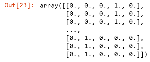
from sklearn.preprocessing import OneHotEncoder
ohe = OneHotEncoder()
df_hot = ohe.fit_transform(ocean)
df_hot

This is called one-hot encoding because only one attribute will be hot, while the rest of them will be cold. These are also dummy attributes.
*Remember the output of this is a spare matrix which really comes in handy when we are dealing with thousands of categories. Because just imagine, if we perform one-hot encoding on an attribute that has thousands of categories we will end up getting a thousand more columns that are full of zeros except a single one per row. Here we are using lots of memory just to store zeros and it is extremely wasteful. So what a sparse matrix does is it stores the locations of all non-zero elements only.
But still, if you want to convert it to NumPy array just call the toarray() method.
df_hot.toarray()
4. Feature Scaling:

Use an equal amount of each ingredient
This is one of the most important transformations that you will need to apply to your data. Generally, machine learning algorithms don’t perform well when the numerical attributes are not having the same scale.
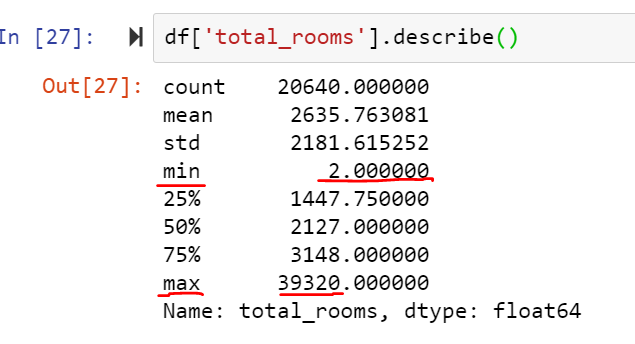
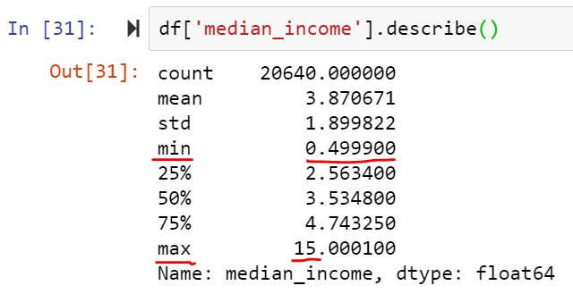
In our dataset, we can see that the median income ranges only from 0 to 15 whereas the total number of rooms ranges from about 2 to 39,320.
So now we have two ways through which we can get all attributes on the same scale:
- Min-Max Scaling.
- Standardization.
Min-Max Scaling:
Also known as, Normalization and is one of the simplest scalers. Here what this transformer does is it shifts and rescales the values so that they end ranging from 0-1. This is done by subtracting the minimum value and dividing it by the differences between maximum and minimum value.

Sckit-Learn has a transformer for this task, MinMaxScaler and it also has a hyperparameter called feature_range which helps in changing the range, if for some reason you don’t want the range to be from 0 to1.
Standardization:
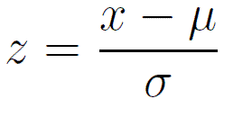
This is a little bit different. What it does is it first subtracts the mean value and after that, it divides it by the standard deviation to get a unit variance.
Here, it does not bound values to some fixed specific range like min-max scalers. This may be a problem with some of the algorithms. For example, Most of the time, Neural Networks excepts an input value ranging from 0 to 1. But there is an advantage of this transformer too! It is not much affected by the outliers. Let’s suppose that median income had a value of 1000 by mistake: Min-Max Scaler will directly rescale all the values from 0-15 to 0-0.015, whereas standardization won’t be affected.
Sckit-Learn has a transformer for this task, StandardScaler.
5. Transformation Pipelines:

As of today, we saw that there are a lot of data transformation steps involved in data pre-processing that must be performed in the right order. The good news is Sckit -Learn has an amazing class for this tedious task to be effortless, it is called the Pipeline class and helps with managing the sequence of this task.
Let me show what I mean by that:
from sklearn.pipeline import Pipeline
from sklearn.preprocessing import StandardScaler
pipe = Pipeline([
    ('imputer',SimpleImputer(strategy="median")),
    ('std_scaler',StandardScaler())
])
df_tr = pipe.fit_transform(imputer_df)
What this pipeline constructor does is, it takes the list of all the estimators in sequential order. But the last estimator must be a transformer i.e. they should a fit_transform() method. So when we call the pipeline fit transform method, fit_transform is called for every transformer sequentially passing the output of each into its consecutive call and this happens until the fit() method is called(Our final estimator).
In our code, we can see that our last estimator is Standard Scaler, which we know is a transformer. Hence, the pipeline has a transform() method that is applied to all the transformers in sequence.
Conclusion:

Key to make the perfect dish lies in choosing the right and proper ingredients!
Technically what I mean by the above quote is, if you properly preprocess your data your algorithm will definitely be accurate enough to provide the best results on real data. This is the most important that you should take into considerations while building your data science project.
Today, In this article we discussed what and why do we need data pre-processing, what are the several benefits that we get if we make functions while preparing the data, and a couple of methods of data preprocessing. Also, do check out the official documentation of each and every transformer we used to get a tighter grip on them.
Stay tuned!!
I hope enjoyed reading the article. If you found it useful, please share it among your friends on social media too. For any queries and suggestions feel free to ping me here in the comments or you can directly reach me through email.
Connect me on LinkedIn
https://www.linkedin.com/in/karanpradhan266
Email: [email protected]
Thank You !!
The media shown in this article on data pre-processing is not owned by Analytics Vidhya and are used at the Author’s discretion.


