This article was published as a part of the Data Science Blogathon
Welcome readers to Part 2 of the Linear predictive model series. If you haven’t read Part 1 of this series, you can read that here:
Linear Predictive models – Part 1 by Barney6
As a quick recap, in part 1 we obtained our data by web scraping AutoScout24 and obtained the dataset of car sales in Germany. Next, we cleaned and prepared the data for a preliminary Exploratory data analysis. Then we began with our modeling and used several Regression models like Linear regression with and without regularization, Linear regression with Regu, Pipeline, Cross Val Predict, and lastly with Polynomial regularization.
What is Regression in Machine Learning?
Regression analysis can be described as a way of predicting the future of a dependable (target) variable use single or multiple independent variables(also known as predictors). Some examples may be finding the relation between the price of a house, and how big the house is, or using a business example, how the sales are affected due to negative or positive media coverage of the company.
Regression is the most basic and fundamental algorithm of Machine learning. The difference between regression and classification models is that regression models are used to predict a numeric value, whereas classification models are used to divide the obtained data into two or multiple classes or groups.
Some of the important applications of regression are forecasting, time series modeling, and finding the cause and effect relationship between variables.
Why is it important?
The regression analysis has a wide range of real-life and practical applications. Any machine learning problem with a continuous number range – this includes, but is not limited to, a host of examples like:
- Financial forecasting
- Sales and promotions forecasting
- Testing automobiles
- Weather analysis and prediction
- Time series forecasting
Different types of Regression
There are 5 types of regression in total:
- Linear Regression
- Logistic Regression
- Polynomial Regression
- Lasso Regression
- Ridge regression
Let us give a brief definition of all of them:
1) Linear Regression: This is the most basic regression model in machine learning. It comprises a predictor variable and a dependent variable, which are linearly dependent on the former. It involves the use of the best fit line.
One should use Linear Regression when the variables are linearly related. However, this model is susceptible to outliers, so the bigger the data higher the chances of faulty predictions.
2) Logistic Regression: If the dependent variable has a discrete value, in other words, if it can only have one of the two values(either 0 or 1, True or False, spam or not spam, etc), then Logistic regression is your best option.
The sigmoid function is used by the Logistic regression to show the relationship between target and independent variables. However, one should keep a few things in mind before using logistic regression: It works best with huge datasets with almost equal occurrences of both classes, and should not contain a high correlation between the independent variables.
3) Polynomial Regression: Polynomial regression tries to model a non-linear dataset to a linear model. It can be thought of as making a square peg fit into a round hole. Polynomial regression works best when the data points are present in a non-linear fashion.
What the model does is transform these non-linear datapoints into polynomial features of a given degree, and then models them using a linear model, however, this regression is most prone to overfitting, so one is advised to analyze curve ends to avoid odd-looking results
4) Ridge Regression: Since we cannot use logistic regression for variables with multicollinearity, our best choice has to be ridge regression. It is a regularization technique to lower the complexity of the model. However, this too is susceptible to overfitting as the ridge uses a bias matrix( known as ridge regression penalty), which introduces a small amount of bias.
5) Lasso Regression: Similar to ridge regression, lasso regression is also a regularization technique used to lower the complexity of a model. it does so by making the coefficient value close to zero, which does not happen in the case of ridge regression.
Lasso regression avoids overfitting by letting the user select a few features from the dataset to build the model.

In the previous article, we worked with different forms of Linear regression, and in this one, we shall work with Lasso and Ridge regression. We will be using the same vehicular dataset which we used priorly.
You can download the dataset here. Since we have already done EDA on our dataset in the previous article, we shall not waste much time doing so again. We’ll just load the data, do the basic analysis, and get started with our modeling. If you wish to see the exploratory data analysis, you can do so from the above link for the previous article.
Loading Data
First, we import the necessary libraries:
import os
import pandas as pd
import numpy as np
import seaborn as sns
import matplotlib.pyplot as plt

from pandas_profiling import ProfileReport
import warnings
warnings.filterwarnings("ignore")
import pandas as pd
df = pd.read_csv("autoscout24-germany-dataset.csv")
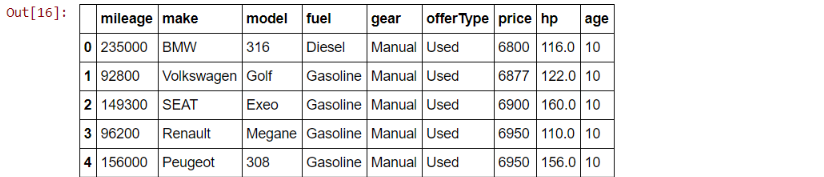
print(df.head())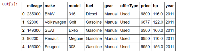
‘Price” is our target variable.
Getting Familiar with the data
df.shape
> (46405, 9)
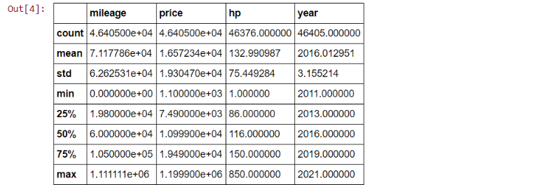
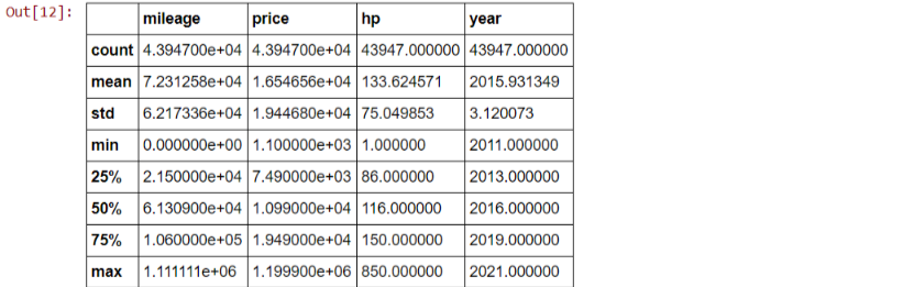
df.describe()
df['fuel'].unique()

df['gear'].unique()
> array(['Manual', 'Automatic', nan, 'Semi-automatic'], dtype=object)
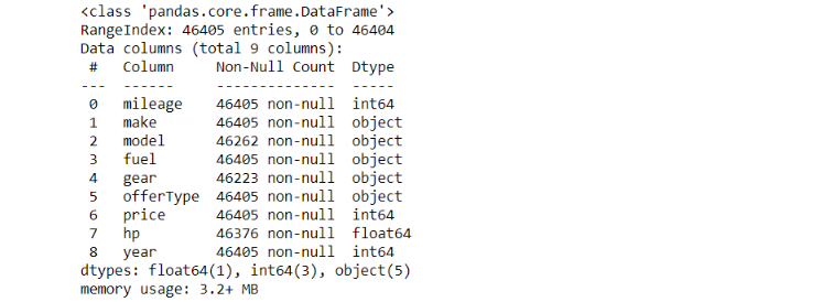
df.info()
Now time for preparing the data. We shall omit the entries with null values since there are only a few of them.
Data Cleaning and Preparation
df.isna().sum()
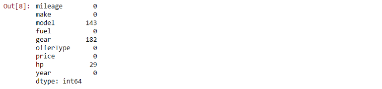
Since the amount of missing values is less than 1% of our total data, we can drop these entries without many problems.
df.dropna(inplace = True)
#dropping duplicate rows
df.drop_duplicates(keep = 'first', inplace = True)
#now let's see the shape of our dataframe df.shape
> (43947, 9)
df.describe()
Using the column ‘Year’ to find the age of the vehicles.
from datetime import datetime
df['age'] = datetime.now().year - df['year']
df.drop('year',axis = 1, inplace = True)
df.head()
Now we continue with our modeling from the previous article.
But first, let us get more familiarised with both the regression types and how they differ or are better from the conventional regression models:
Ridge Regression
Ridge regression is the best candidate to use while faced with the problem of multicollinearity and uses the L2 Regularization. The problem with multicollinearity is that least-squares are unbiased, and variances are very large, which results in a significant difference between the predicted and the actual values.
The cost function used is:
Min(||Y – X(theta)||^2 + λ||theta||^2)
where lambda is the penalty term. The lambda(λ) given here is denoted by an alpha parameter in the ridge function. Thus we can control the penalty term by changing the values of alpha. The higher the value of alpha, the higher is the penalty and thus the magnitude of coefficients is reduced.
Therefore we can say that it shrinks the parameters, which ultimately prevents multicollinearity and also reduces the model complexity.
If you want to read more in-depth about ridge regression, you can check out these articles:
Ridge Regression: Simple Definition by Statistics How to
What is Ridge Regression? by Great Learning
Lasso Regression
LASSO stands for Least Absolute Shrinkage Selector Operator. It is also a regularization technique like Ridge regression, to combat overfitting and have more accurate results.
The mathematical equation is:
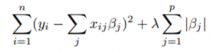
Lasso uses something called Shrinkage. Shrinkage is when the data points are shrunk into a central point like mean. The lasso procedure encourages simpler models with fewer parameters. Lasso uses L1 regularization.
What L1 regularization does is add a penalty that is equal to the absolute value of the magnitude of the coefficients. Some of these coefficients might become zero and get eliminated. This elimination does not occur in L2 regularization, making Lasso easier to interpret as compared to Ridge.
Here are 2 great videos that’ll help you build a better intuition and showcase the difference between Ridge and Lasso.
Modeling
Everything we did until this point, is to prepare our data for modeling. Now we will implement various versions of Lasso Regression and Ridge regression to see which model has the most accuracy.
1) Lasso Regression with Regularization
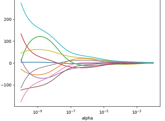
Image Source: Jan Kirenz, Lasso regression with Python
import numpy as np
alphas = np.geomspace(1e-9, 1e-0, num=10)
alphas
from sklearn.linear_model import Lasso
scores_lasso = []
coefs = []
for alpha in alphas:
las = Lasso(alpha=alpha, max_iter=100000)
estimator = Pipeline([('scaler', s), ('lasso_regression', las)])
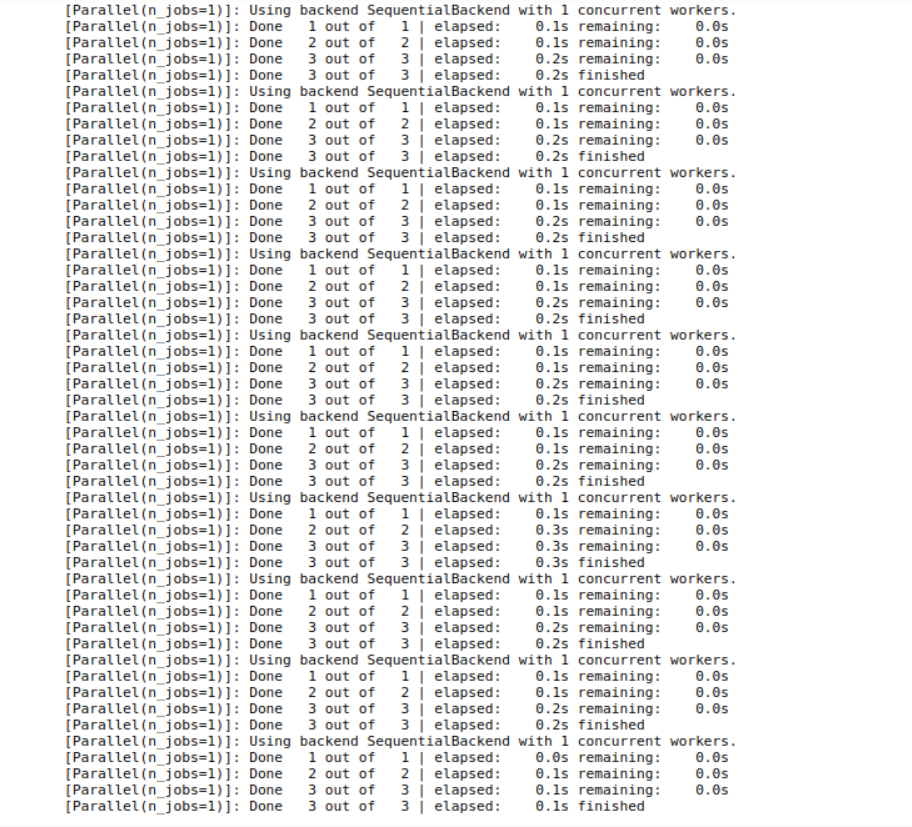
predictions = cross_val_predict(estimator, X, y, cv=kf, verbose=100)
score = r2_score(y, predictions)
scores.append(score)
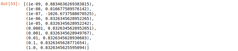
list(zip(alphas, scores))
Lasso(alpha=1e-6).fit(X,y).coef_

Lasso(alpha=1).fit(X,y).coef_

2) Lasso Regression with Polynomial Regularization
from sklearn.preprocessing import PolynomialFeatures
from sklearn.linear_model import Lasso
from sklearn.model_selection import KFold
pf = PolynomialFeatures(degree=3)
scores = []
alphas = np.geomspace(9, 12, 4)
# alphas = np.geomspace(0.001, 10, 5)
for alpha in alphas:
las = Lasso(alpha=alpha, max_iter=10000)
estimator = Pipeline([('make_higher_degree', pf), ('scaler', s), ('lasso_regression', las)])
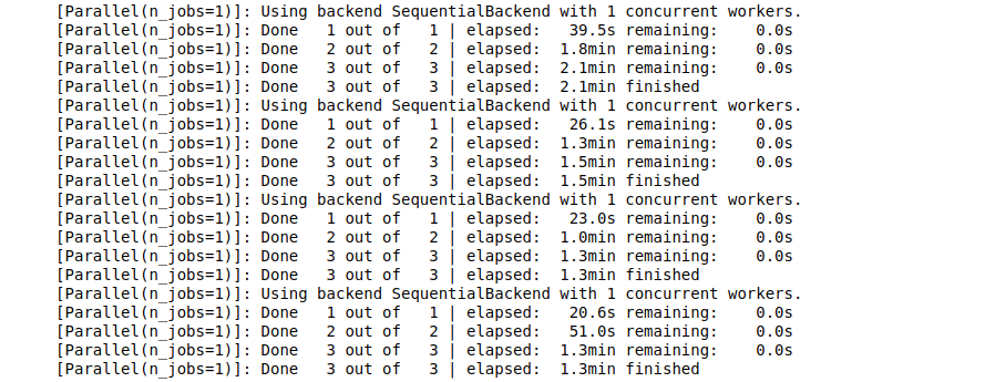
predictions = cross_val_predict(estimator, X, y, cv=kf, verbose=100)
score = r2_score(y, predictions)
scores.append(score)
alphas
> array([ 9.        ,  9.90578175, 10.90272356, 12.        ])
scores
> [0.8792881358296342,  0.8815238961714683,  0.8833873929387192,  0.8846801909901439]
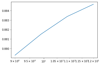
import matplotlib.pyplot as plt
plt.semilogx(alphas, scores)
Lasso regression using the best estimator from above
best_estimator = Pipeline([('make_higher_degree', PolynomialFeatures(degree=2)), ('scaler', s), ('lasso_regression', Lasso(alpha=10, max_iter=100000))])
best_estimator.fit(X,y)
best_estimator.score(X,y)
> 0.8855454953727971
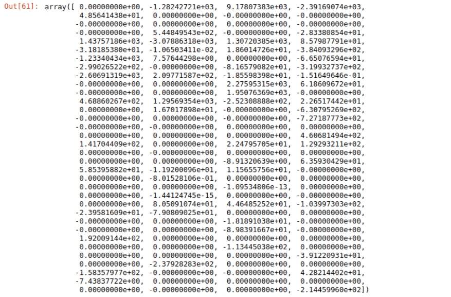
best_estimator.named_steps['lasso_regression'].coef_
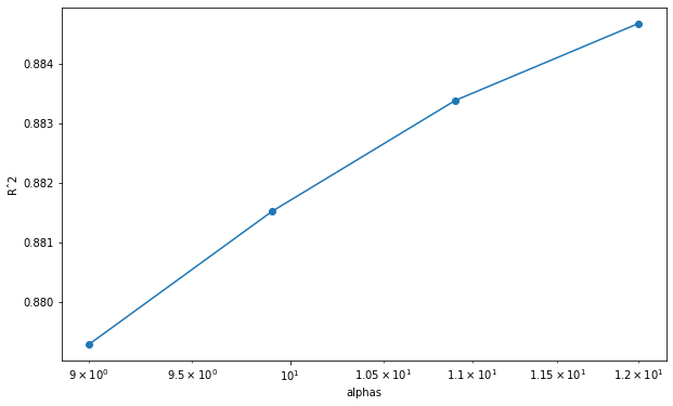
plt.figure(figsize=(10,6))
plt.semilogx(alphas, scores, '-o')
plt.xlabel('alphas')
plt.ylabel('Rˆ2')
3) Ridge Regression
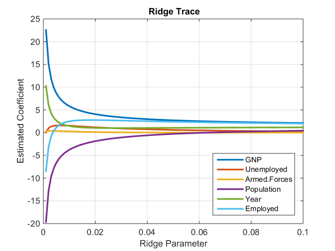
Image Source: Stack Exchange
X.shape
> (40387,15)
y.shape
> (40387,)
from sklearn.linear_model import Ridge
pf = PolynomialFeatures(degree=2)
alphas = np.geomspace(0.1,2,20)
scores=[]
for alpha in alphas:
  ridge = Ridge(alpha=alpha, max_iter=100000)
  estimator = Pipeline([('make_higher_degree', pf), ('scaler', s), ('ridge', ridge)])
  predictions = cross_val_predict(estimator, X, y, cv=kf, verbose=100)
  score=r2_score(y, predictions)
  scores.append(score)
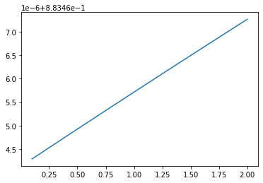
plt.plot(alphas, scores)
best_estimator = Pipeline([('make_higher_degree', PolynomialFeatures(degree=2, include_bias=False)), ('scaler', s), ('lasso_regression', Lasso(alpha=10))])
best_estimator.fit(X,y)
best_estimator.score(X,y)
> 0.8855454953727971
Therefore we can see that we get an accuracy of around 88.5% using both of our regularization techniques which is a much better result than the 83.9% from using only Linear regression in our previous article.
End Notes
Thanks for reading this article. This is the conclusion for the 2 part series on Linear predictive models. If you enjoyed reading this, be sure to check out my other articles on:
Barney6, Author at Analytics Vidhya
You can read another article by Analytics Vidhya which was an inspiration for me to write these articles:
Comprehensive beginners guide for Linear, Ridge, and Lasso Regression in Python and R by Subham Jain
Here is the Github link for the code for this article:


