This article was published as a part of the Data Science Blogathon
Introduction
In one of my previous articles, I have explained the concept of Modules in Python. If you haven’t read that article, then please refer to that article first and then read this article in continuation to that since in this article we will discuss the applications of the Random Python Module which involves somehow understanding of the basic concept involved in Modules.

Image Source: Link
In this article, we use the Random module of Python to visualize some of the common probability distributions and observe the need of learning some important python modules in a Data Science Journey. So, If you are a Data Science enthusiast, then read this article completely and accelerate your Data Science Journey to become Data Scientist.
Table of Contents
The topics which we are going to discuss in this article are as follows:
- What is a Random Number?
- What is a Probability Distribution?
- Visualizing and Understanding Normal Distribution
- Visualizing and Understanding Poisson Distribution
- Visualizing and Understanding Binomial Distribution
What is a Random Number?
The random number doesn’t mean a unique number anytime. Random means something that may not be predicted logically.
There are two types of Random Numbers:
- Pseudo-Random, and
- True Random
Computers work on programs, and programs are a definitive set of instructions. So it means there must be some algorithm to come up with a random number further.
If there’s a program to come up with a random number it is often predicted, thus it’s not truly random. When we generate random numbers through a generation algorithm, then those random numbers are called pseudo-random.
What is a Probability Distribution?
A probability distribution gives us a law according to which different values of the random variable are distributed with some specified probability. So, a probability distribution is a set of all possible values that a random variable can take, along with the associated probability of each.
In this article, we will be discussing the following probability distributions:
- Normal Distribution
- Poisson Distribution
- Binomial Distribution
Normal Distribution
The normal distribution is one of the most used distributions in Data Science since many common phenomena that take place in our daily life follow a normal distribution. It is also known as the Gaussian Distribution and is famous for its bell shape. The curve for this distribution is symmetrical about the mean. The normal distribution is a continuous distribution. It fits the probability distribution of the many events.
The Mean, Median, and Mode of the normal distribution coincide with each other, and also, the skewness of the curve is zero.
For Example, Some of the examples of normal distribution in our daily lives are as follows:
- The income distribution in the economy,
- The students’ average marks,
- The average height of individuals in a country.
The Probability density function (PDF) of a random variable X following a normal distribution is given by:
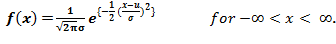
The curve of a random variable X ~ N (µ, σ) is shown below:
Image Source: Link
The standard normal distribution is defined as the normal distribution with mean 0 and standard deviation 1. For such a case, the probability density function (PDF) becomes:

And, the curve for standard normal distribution is shown below:

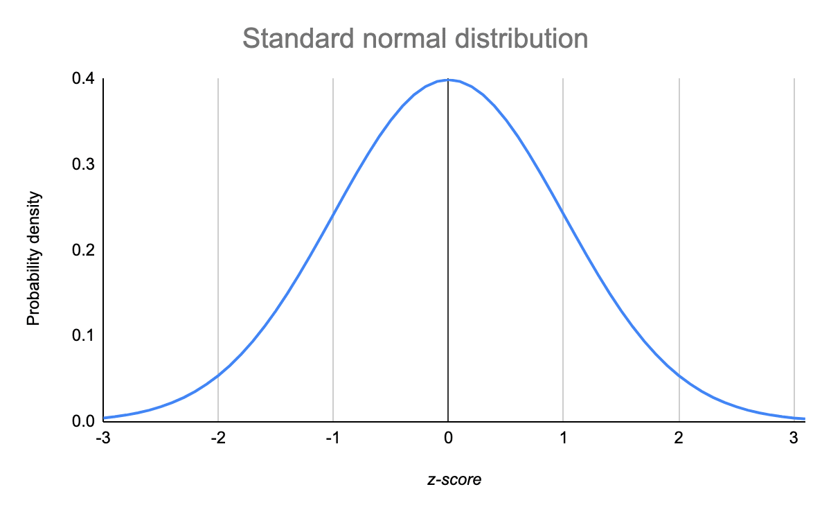
Image Source: Link
To generate a standard Normal Data distribution, we use the random.normal() method.
To implement this distribution using NumPy, we have to input the following three parameters:
- loc parameter: describes the Mean value i.e, where the height of the bell exists.
- scale parameter: describes the Standard Deviation i.e, how flat the graph distribution should be.
- size parameter: return the shape of the output array.
For Example –
Generating a random array of size 3 by 3 and the data inside that array comes from a normal distribution having mean equals zero and standard deviation equal to one i.e, Standard Normal Distribution.
from numpy import random
array = random.normal(loc=0, scale=1, size=(3, 3))
print(array)
The output that I got after the successful execution of the above program is shown below: (In My Local Machine)
[[ 2.13114217  2.74524848 -0.69011481]
 [ 0.22094458 -0.67127781 -1.72408367]
 [-0.97152815  1.49916247  1.54961289]]
For Example –
Generate a normal distribution having mean equals zero and standard deviation equals one using the random module of Python.
from numpy import random

import matplotlib.pyplot as plt

import seaborn as sns

sns.distplot(random.normal(loc=0, scale=1, size=200), kde=True)

plt.show()
The output that I got after the successful execution of the above program is shown below: (In My Local Machine)
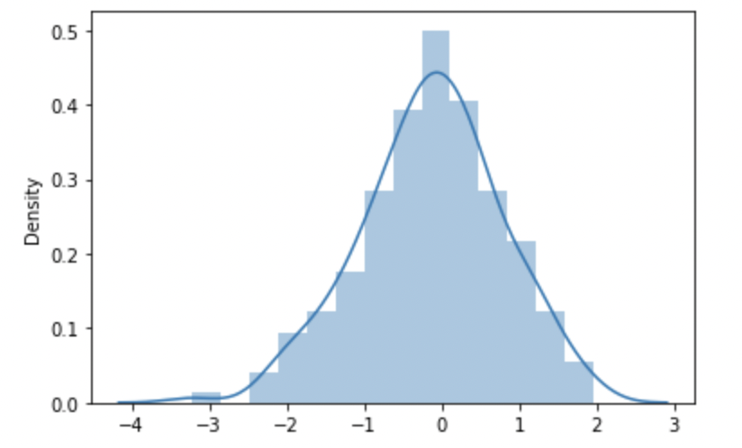
Image Source: Author
Poisson Distribution
Poisson distributions are commonly used to find the probability that an event might happen or not, knowing often it usually occurs. It is basically used to model the frequency with which a specific event occurs over a period of time or interval.
Poisson Distribution is a Discrete Distribution. It estimates how many times an occurrence can happen in an exceedingly specified time.
For Example, Some of the examples of Poisson distribution in our daily lives are as follows:
- The number of emails arriving in your inbox in one hour,
- The number of customers going into a shop in one week.
- If someone eats twice daily what probability will he eat thrice?
Since this is a discrete distribution, so the probability mass function (PMF) of random variable X following a Poisson distribution is given by:
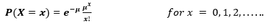
For this distribution, the mean µ is the parameter and is also defined as the λ times the length of that interval. So, the curve of a Poisson distribution is shown below:

In the graph shown below, we illustrate that the shift in the curve is due to an increase in the value of the mean.
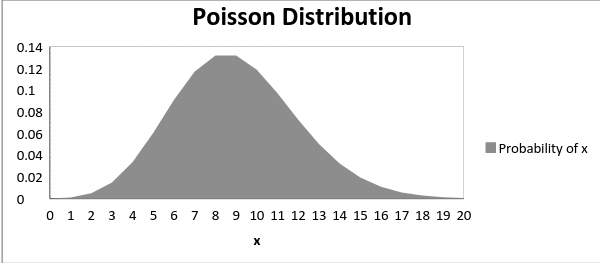
Image Source: Link
Therefore, It is true that as the mean increases, then the curve shifts to the right.
To generate a Poisson distribution, we use the random.poisson() method.
To implement this distribution using NumPy, we have to input the following two parameters:
- lam parameter: describes the rate or known number of occurrences
- size parameter: return the shape of the output array.
For Example –
Generating a random array of size 1 by 5 and the data inside that array comes from a Poisson distribution having occurrence equals to 5.
from numpy import random
array = random.poisson(lam=5, size=5)
print(array)
The output that I got after the successful execution of the above program is shown below: (In My Local Machine)
[4 3 5 4 5]
For Example –
Generate a Poisson distribution having occurrence equals 5 using the random module of Python.
from numpy import random
import matplotlib.pyplot as plt
import seaborn as sns
sns.distplot(random.poisson(lam=5, size=200), kde=True)
plt.show()
The output that I got after the successful execution of the above program is shown below: (In My Local Machine)
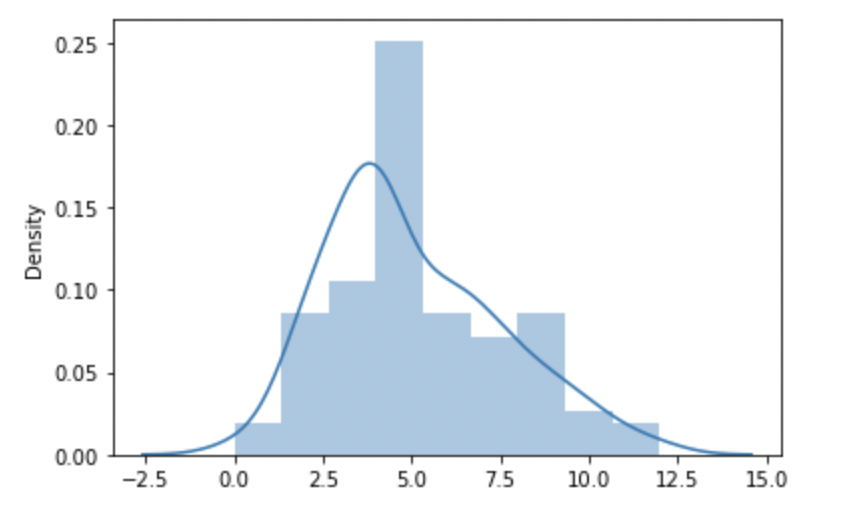
Image Source: Author
Binomial Distribution
Binomial Experiment is basically ‘n’ Bernoulli trials, where n is greater than one i.e, n>1. It denotes the probability of ‘x’ successful trials and consequently, ‘(n-x)’ failures in n number of independent trials.
Here, if you are a beginner, then you might think what a Bernoulli Trials are. So. let’s discuss the Bernoulli trials with the help of a Bernoulli distribution.
A random experiment whose outcomes are of two types, a success S and a Failure F, occurring with probabilities p and q respectively, is called a Bernoulli Trial. For Example, Tossing a coin.
Binomial Distribution is a Discrete Distribution. It describes the result of binary scenarios.
For Example, Tossing 10 coins simultaneously.
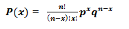
The mathematical expression involved in binomial distribution is shown below:
Following is a binomial distribution graph where the probability of success and the probability of failure does not equal.

Now, when the probability of success = probability of failure, in such cases, the graph of the binomial distribution is shown below:
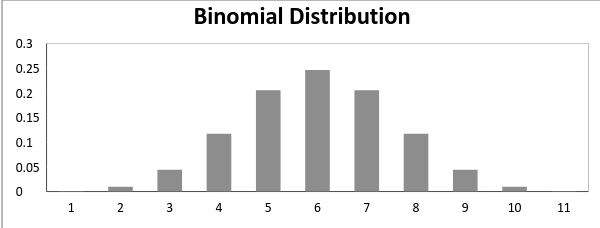
Image Source: Link
To generate a Binomial distribution, we use the random.binomial() method.
To implement this distribution using NumPy, we have to input the following three parameters:
- n parameter: denotes the number of trials.
- p parameter: describes the probability of occurrence of every trial.
- size parameter: return the shape of the output array.
For Example –
Generate a random array of 5 data points for a given 5 trials for a fair coin toss.
from numpy import random
array = random.binomial(n=5, p=0.5, size=5)
print(array)
The output that I got after the successful execution of the above program is shown below: (In My Local Machine)
[3 2 2 5 3]
For Example –
Generate a Binomial distribution for a given 5 trials of a fair coin toss using the random module of Python.
from numpy import random
import matplotlib.pyplot as plt
import seaborn as sns
sns.distplot(random.binomial(n=5, p=0.5, size=200), hist=True, kde=False)
plt.show()
The output that I got after the successful execution of the above program is shown below: (In My Local Machine)
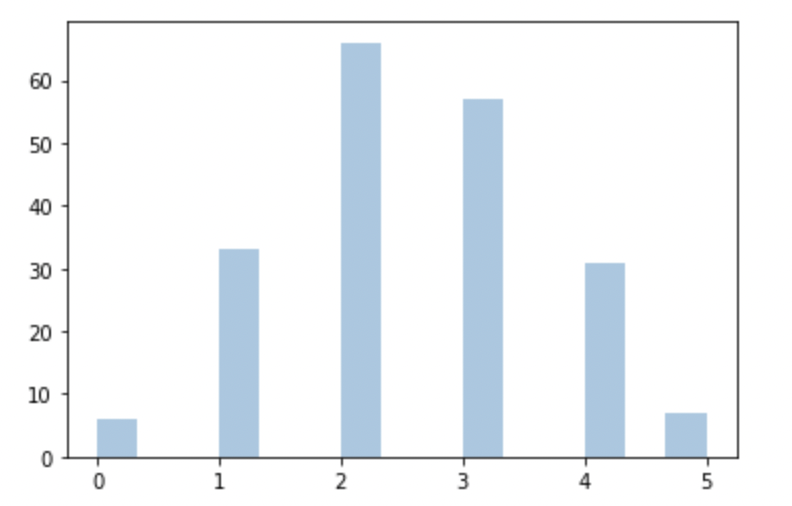
Image Source: Author
Self Learning Resource
If you want to know in deep about all the probability distributions that are commonly used in Data Science, then refer to the following link:
Understanding all Probability Distributions
Other Blog Posts by Me
You can also check my previous blog posts.
Previous Data Science Blog posts.
Here is my Linkedin profile in case you want to connect with me. I’ll be happy to be connected with you.
For any queries, you can mail me on [email protected]
End Notes
Thanks for reading!
I hope that you have enjoyed the article. If you like it, share it with your friends also. Something not mentioned or want to share your thoughts? Feel free to comment below And I’ll get back to you. 😉
I am a B.Tech. student (Computer Science major) currently in the pre-final year of my undergrad. My interest lies in the field of Data Science and Machine Learning. I have been pursuing this interest and am eager to work more in these directions. I feel proud to share that I am one of the best students in my class who has a desire to learn many new things in my field.


