Perform Logistic Regression with PyTorch Seamlessly

This article was published as a part of the Data Science Blogathon

Regression has numerous applications in real life. Linear regression is used to predict continuous variables. For example, if you want to predict the selling price of a house based on square footage, area of location, no of rooms, etc, you can use Linear Regression. But in some cases, we don’t want to predict a number, but we want to allot a category. For example, given the medical information data of a population, we want to classify them into cancer-affected patients or healthy people.

These are 2 classes. Here, we use logistic regression. Other examples include email classification as spam/not spam etc.

Source

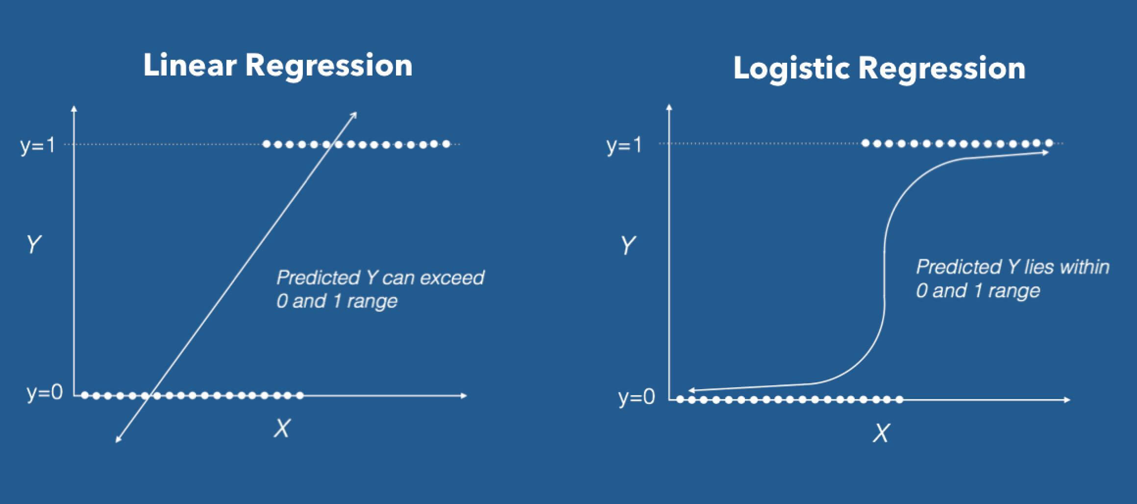
In short, the target variable we want to predict in logistic regression is not continuous, it’s discrete. An example where logistic regression can be applied is email classification: Identity as Spam or not spam. Image classification, text classification all fall into the category.

I assume you are familiar with implementing logistic regression using the sklearn library. In this blog, we shall see how to implement logistic regression in PyTorch. This will help you if you trying to learn PyTorch. I’ll cover what are the steps to solve a problem in PyTorch while explaining every term.

Grab a coffee and charge up to de-mystify Pytorch!

1. Dataset loading

Here, I’ll be using the Breast cancer dataset from the sklearn library. This is a simple binary class classification dataset. You can load it from sklearn.datasets module. Next, you can extract X and Y from the dataset using the inbuilt function as shown below.
Python Code:

from sklearn import datasets
breast_cancer=datasets.load_breast_cancer()
x,y=breast_cancer.data,breast_cancer.target
print(x)

x is the data with all features, while y has the target or the class. Next, we should find the size of the dataset and what is the no of features in x. The below code executes it in one line.

n_samples,n_features=x.shape
print(n_samples)
print(n_features)
#> 569 
#> 30

So, we know the dataset has 569 samples and 30 features. Next, we will split it into training and testing batches using sklearn’s “train_test_split”. This can be imported from the model selection module.

from sklearn.model_selection import train_test_split
x_train,x_test,y_train,y_test= train_test_split(x,y,test_size=0.2)

In the above code, test size denotes the fraction of data you want to use as a test dataset. So, 80% for training and 20% for testing.

2. Preprocessing

Since this is a classification problem, a good preprocessing step would be to apply standard scaler transformation.

scaler=sklearn.preprocessing.StandardScaler()
x_train=scaler.fit_transform(x_train)
x_test=scaler.fit_transform(x_test)

Now, there is a last and crucial step of data processing before moving to models. Pytorch works with tensors. So, we convert all four into tensors using the “torch.from_numpy()” method. It is important to convert the datatype into float32 before this. You can do that using “astype()” function.

import numpy as np
x_train=torch.from_numpy(x_train.astype(np.float32))
x_test=torch.from_numpy(x_test.astype(np.float32))
y_train=torch.from_numpy(y_train.astype(np.float32))
y_test=torch.from_numpy(y_test.astype(np.float32))

But, we know that y has to be in the form of a column tensor and not a row tensor. We perform this change using the “view” operation as shown in the code. Do the same operation for y_test also.

y_train=y_train.view(y_train.shape[0],1)
y_test=y_test.view(y_test.shape[0],1)

The preprocessing steps are completed, you can move ahead to model building.

3.Model Building

Now, we have the input data ready. Let’s see how to write a custom model in PyTorch for logistic regression. The first step would be to define a class with the model name. This class should derive torch.nn.Module.

Inside the class, we have the __init__ function and forward function.

class Logistic_Reg_model(torch.nn.Module):
 def __init__(self,no_input_features):
   super(Logistic_Reg_model,self).__init__()
   self.layer1=torch.nn.Linear(no_input_features,20)
   self.layer2=torch.nn.Linear(20,1)
 def forward(self,x):
   y_predicted=self.layer1(x)
   y_predicted=torch.sigmoid(self.layer2(y_predicted))
   return y_predicted

In the __init__ method, you have to define the layers you want in your model. Here, we use Linear layers, which can be declared from the torch.nn module. You can give any name to the layer, like “layer1” in this example. So, I have declared 2 linear layers.

The syntax is: torch.nn.Linear(in_features, out_features, bias=True)

Next, we have the “forward()” function which is responsible for performing the forward pass/propagation. The input is passed through the 2 layers defined earlier. In addition, the output from the second layer is passed through an activation function called sigmoid.

What is an activation function?

Activation functions are used to capture the complex relationships in linear data. In this case, we use a sigmoid activation function.

The reason we have chosen the sigmoid function, in this case, is because it will restrict the value to (0 to 1). Below is a graph of sigmoid function along with its formula

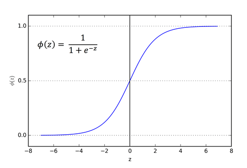
Source: Imagelink

4. Training and optimization

After defining the class, you can initialize a model.

model=Logistic_Reg_model(n_features)

Now, we need to define the loss function and optimization algorithm. Luckily in Pytorch, you can choose and import your desired loss function and optimization algorithm in simple steps. Here, we choose BCE as our loss criterion.

What is BCE loss?

It stands for Binary Cross-Entropy loss. Its usually used for binary classification examples. A notable point is that, when using the BCE loss function, the output of the node should be between (0–1). We need to use an appropriate activation function for this.

For optimizer, we choose SGD or Stochastic gradient descent. I assume you are familiar with the SGD algorithm, which is commonly used as an optimizer. There are other optimizers like Adam, lars, etc. Depending upon the problem, you have to decide on the optimizer. For optimizer, you should give model parameters and learning rate as input.

What is a learning rate?

Optimization algorithms have a parameter called the learning rate. This basically decides the rate at which the algorithm approaches the local minima, where the loss will be minimal. This value is crucial.

Source: Imagelink

 Because if the value is too high, the algorithm might shoot up and miss the local minima. On the other hand, if it’s too small, it will take a lot of time and may not converge. Hence, the Learning rate “lr” is a hyperparameter that should be fine-tuned to an optimal value.

criterion=torch.nn.BCELoss()
optimizer=torch.optim.SGD(model.parameters(),lr=0.01)

Next, you decide the number of epochs and we write the training loop.

number_of_epochs=100
for epoch in range(number_of_epochs):
 y_prediction=model(x_train)
 loss=criterion(y_prediction,y_train)
 loss.backward()
 optimizer.step()
 optimizer.zero_grad()
 if (epoch+1)%10 == 0:
   print('epoch:', epoch+1,',loss=',loss.item())

Here, the first forward pass happens. Next, the loss is calculated. When loss.backward() is called, it computes the gradient of the loss with respect to the weights (of the layer). The weights are then updated by calling optimizer.step(). After this, the weights have to be emptied for the next iteration. So the zero_grad() method is called.

The above code will print the loss at each 10th epoch.

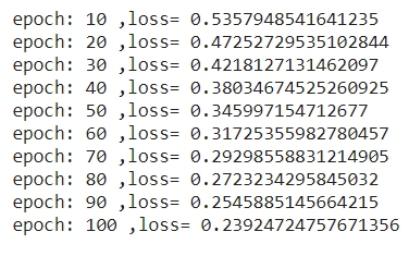
Source: Screenshot from my Jupiter notebook

If you observe the loss is decreasing with the epoch, the algorithm is working right. You can finetune the no of epochs and learning rate and try to improve the performance of the model!

5. Calculate Accuracy

How can you calculate accuracy?

with torch.no_grad():
 y_pred=model(x_test)
 y_pred_class=y_pred.round()
 accuracy=(y_pred_class.eq(y_test).sum())/float(y_test.shape[0])
 print(accuracy.item())

We have to use torch.no_grad() here. The aim is to basically skip the gradient calculation over the weights. So, whatever I write inside this loop will not cause a change in the weights and hence not disturb the backpropagation process. In this case, I got an accuracy of 0.92105!

Hope this was useful. Thanks for the read!

Connect with me over email: [email protected]