This article was published as a part of the Data Science Blogathon
Introduction
Indian Premier League or as it is famously known IPL is one of the most loved cricket championships across the world. It was started in 2007 by the BCCI in India having 20-20 cricket formats and eight teams. Teams can have national or international players. This was the main game-changer in this championship since players from different national teams can now play together which many fans have wanted to see for a long time.
There are eight teams in IPL that were introduced at the beginning which are as follows:
- Bangalore Royal Challengers
- Chennai Super Kings
- Deccan Chargers
- Delhi Daredevils
- Kings XI Punjab
- Kolkata Knight Riders
- Mumbai Indians
- Rajasthan Royals
An auction was held initially to decide the ownership of teams for the time period of 10 years with a base price of USD 50 million. There are several rules that are imposed by IPL that need to be followed to be in an IPL team. For example, Only international and famous Indian players are auctioned. Each player has a base price which is decided by various performance metrics. Even though IPL follows the 20-20 cricket format it is possible that the base price of a player is influenced by the performance of players in other cricket formats line One-Day-International(ODI) and Test-Match.
In this article, we will try to predict the selling price of a player given their past performances in other cricket formats. The data we will be using have information of 130 players who played in at least one season of IPL from 2008 till 2011.
Developing Multiple Linear Regression Model with Machine Learning
In this section, we will be discussing various steps involved in developing a multiple linear regression model using python.
- Loading dataset
- Displaying the first five records
- Encoding Categorical Features
- Splitting the dataset into train and validation sets
- Building the Model on the Training Dataset
- Multi-Collinearity and Handling Multi-Collinearity
- Build a new model after Removing Multi-collinearity
Lets’ go
1. Loading the dataset
Loading data from here IPL IMB381IPL2013.csv the file and print the metadata.
import numpy as np
import pandas as pd
ipl_au=pd.read_csv("IPL IMB381IPL2013.csv")
ipl_au.info()
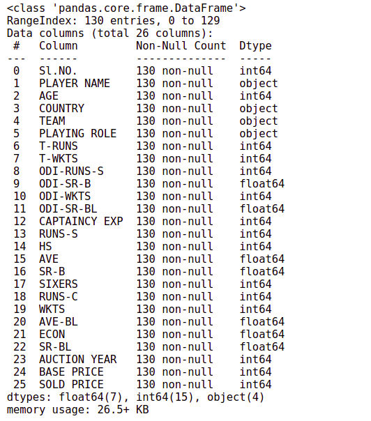
There are 130 observations and 26 columns in the data, and there are no missing values.
2. Displaying first five records
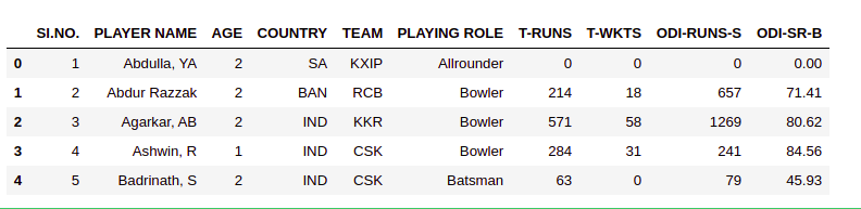
As the number of columns is very large, we will display the initial 10 columns for the first 5 rows. The function ‘iloc()’ is used for displaying a subset of the dataset.
ipl_au.iloc[0:5,0:10]
We can build a model to understand what features of players are influencing their sold price or predict the player’s auction price in future.
we will create a variable x_features which will contain the list of features that we will finally use for building the model and ignore the rest of the columns of the dataframe. The following function is used for including the features in the model building.
x_features=ipl_au.columns
Most of the features in the dataset are numerical whereas features such as age, country, playing-role, captaincy-exp are categorical and hence need to be encoded before building the model.
x_features=['AGE','COUNTRY','PLAYING ROLE','T-RUNS','T-WKTS','ODI-RUNS-S','ODI-SR-B',
            'ODI-WKTS','ODI-SR-BL','CAPTAINCY EXP','RUNS-S','HS','AVE','SR-B','SIXERS',
            'RUNS-C','WKTS','AVE-BL','ECON','SR-BL']
Categorical variables can not be directly included in the regression model and they must be encoded using dummy variables before model building. Let’s move to how to do encoding categorical features.
3. Encoding Categorical Features
Categorical variables need to be encoded using dummy variables before building the model. If a categorical variable has n categories then we will need n-1 dummy variables. So in the case of playing-role, we will need three dummy variables since there are four categories. Finding unique values of column playing role shows the values.
ipl_au['PLAYING ROLE'].unique()

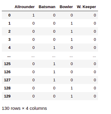
The variable convert into four dummy variables. The can be done using the ‘get_dummy()’ method of ‘pandas’.
pd.get_dummies(ipl_au['PLAYING ROLE'])
we can create dummy variables for all categorical variables present in the dataset.
cate_features=['AGE','COUNTRY','PLAYING ROLE','CAPTAINCY EXP']
ipl_au_encoded_df=pd.get_dummies(ipl_au[x_features],columns=cate_features,drop_first=True)
ipl_au_encoded_df.columns
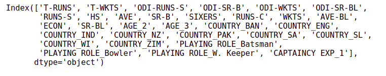
The dataset contains the new dummy variables that have been created. we can reassign the new features to the variable x_features, which we created earlier to keep track of all features that will be used to build the model finally.
x_features=ipl_au_encoded_df.columns
4.Splitting the dataset into train and validation set
Before building the model, we will split the dataset into 80-20 ratios. The split function allows using a parameter random_state, which is a seed function for randomness. Here we will use the random state value is 42.
from statsmodels import api as sm
from sklearn.model_selection import train_test_split
x=sm.add_constant(ipl_au_encoded_df)
y=ipl_au['SOLD PRICE']
X_train, X_test, Y_train, Y_test = train_test_split(x, y, test_size=0.8, random_state=42)
Using another random value may give different training and test data hence different results.
5. Building the Model on the Training Dataset
we will build the Multiple Linear Regression (MLR) model using the training dataset and analyze the model summary. The Summary provides details of the model accuracy, feature significance, and signs of any multi-collinearity effect, which will discuss in detail in the next section.
ipl_model_1=sm.OLS(Y_train,X_train).fit()
ipl_model_1.summary2()
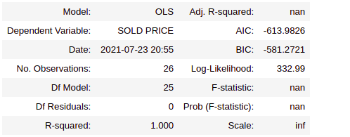

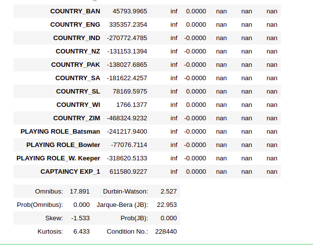
In the MLR model, as per the p-value(<0.05), only the features HS, AGE_2, AVE and Country_ENG have come out significant. The model says that none of the other features is influencing sold price. This is not very intuitive and could be a result of the multi-collinearly effect of variables. For better results, we need to handle multicollinearity. let’s understand what this is?
6. Multi-Collinearity and Handling Multi-Collinearity
When the dataset has a large number of independent variables, it is possible that few of these independent variables may be highly correlated. The existence of a high correlation between independent variables is called multi-collinearity.
The presence of multicollinearity can destabilize the multiple linear regression model. It is necessary to identify the presence of multi-collinearity and take corrective actions.
There are two ways to handle multi-collinearity:-
6.1 Variance Inflation Factor(VIP)
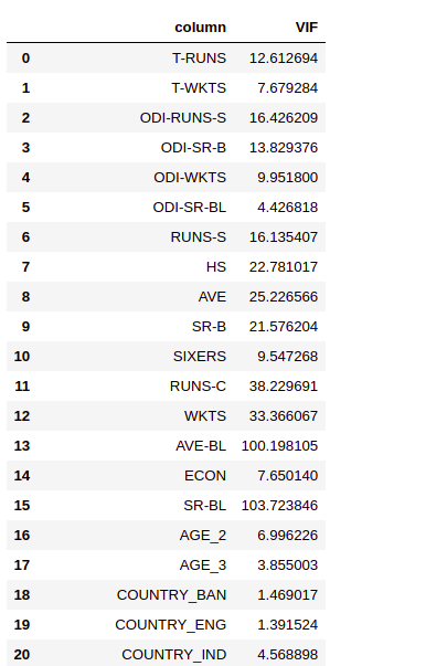
The variance inflation factor is a measure used for identifying the existence of multi-collinearity.
variance_inflation_factore() method available in statsmodels.stats.outliers_influence package can be used to calculate VIF for the features.
from statsmodels.stats.outliers_influence import variance_inflation_factor
def get_vif_factors(x):
    x_matrix=x.to_numpy()
    vif=[variance_inflation_factor(x_matrix,i) for i in range (x_matrix.shape[1])]
    vif_factors=pd.DataFrame()
    vif_factors['column']=x.columns
    vif_factors['VIF']=vif
    return vif_factors
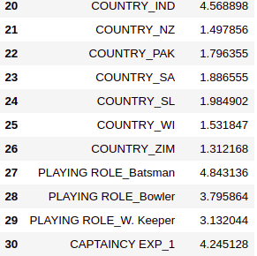
Now, calling the above function with the x features will return the VIF for the corresponding features.
vif_factors=get_vif_factors(x[x_features])
vif_factors
6.2. Checking correlation of columns with large VIFs
We can generate a correlation heatmap to understand the correlation between the independent variables which can be used to decide which features to include in the model. We will first select the features that have a VIF value of more than 4.
columns_with_large_vif=vif_factors[vif_factors.VIF>4].column
Then plot the heatmap for features with VIF more then 4.
import seaborn as sn
import matplotlib.pyplot as plt
plt.figure(figsize=(12,10))
sn.heatmap(x[columns_with_large_vif].corr(), annot = True)
plt.title("heatmap depicting corr between features")
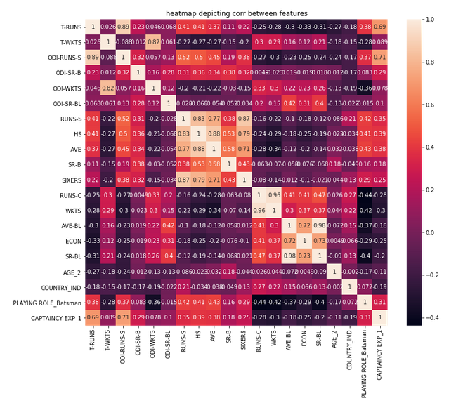
To avoid multicollinearity, we can keep only one column from each group of highly correlated variables and remove the others. We have decided to remove the following features.
columns_to_be_removed = ['T-RUNS','T-WKTS','RUNS-S', 'HS', 'AVE','RUNS-C','SR-B','AVE-BL',
                            'ECON', 'ODI-SR-B','ODI-RUNS-S','SR-BL', 'AGE_2']
x_new_features=list(set(x_features)-set(columns_to_be_removed))
get_vif_factors(x[x_new_features])
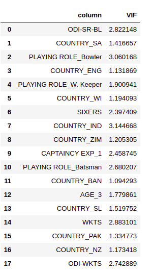
The VIFs on the final set of variables indicate that there is no multicollinearity present anymore. Now we can proceed to build the model with this set of variables now.
7. Build a new model after Removing Multi-collinearity
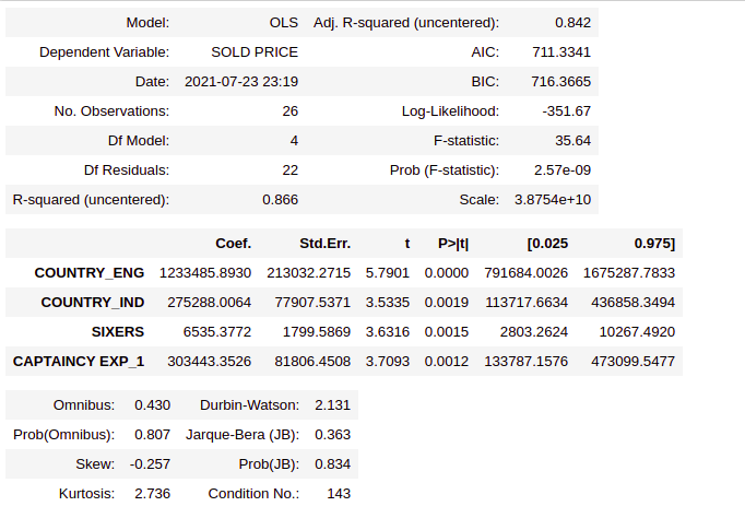
X_train = X_train[x_new_features]
ipl_model_2=sm.OLS(Y_train,X_train).fit()
ipl_model_2.summary2()
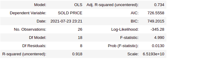
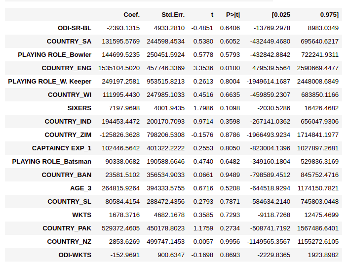

Based on the p- values, only the variables Country_IND, Country_ENG, SIXERS, CAPTAINCY EXP_1 have come out statically significant. So, the features that decide the cold price are
- Players belong to India or the origin country of the player
- How many sixes has the player hit in the previous of the IPL?
- How many wickets have been taken by the player in ODI?
- Player has any previous captaincy experience or not?
Let’s create a new list called significant_vars to store the column name of significant variables and build a new model.
significant_vars=['COUNTRY_ENG','COUNTRY_IND','SIXERS','CAPTAINCY EXP_1']
X_train=X_train[significant_vars]
ipl_model_3=sm.OLS(Y_train,X_train).fit()
ipl_model_3.summary2()
Conclusion
In this article, we learnt how to build, diagnose, understand, and validate the Multiple Linear Regression(MLR) model using python APIs. The multiple Linear Regression(MLR) model is used to find the existence of an association relationship between a dependent variable and more than one independent variable.
In MLR, the regression coefficient is called partial regression coefficient, since they measure the change in the value of the dependent variable for every one unit change in the value of the independent variable when all other independent variables in the model are kept constant. While building the MLR model, categorical variables with N categories should be replaced with (N-1) dummy variables to avoid model misspecification.
Every MLR model should be checked for the presence of multicollinearity since multi-collinearity can destabilize the MLR model.
About the Author
Hi, I am Kajal Kumari. I have completed my Master’s from IIT(ISM) Dhanbad in Computer Science & Engineering. As of now, I am working as Machine Learning Engineer in Hyderabad. You can also check out few other blogs that I have written here.
The media shown in this article on LSTM for Human Activity Recognition are not owned by Analytics Vidhya and are used at the Author’s discretion.
Hi, I am Kajal Kumari. have completed my Master’s from IIT(ISM) Dhanbad in Computer Science & Engineering. As of now, I am working as Machine Learning Engineer in Hyderabad.
hope that you have enjoyed the article. If you like it, share it with your friends also. Please feel free to comment if you have any thoughts that can improve my article writing.
If you want to read my previous blogs, you can read Previous Data Science Blog posts here. Connect with me


