Introduction

In this article, we’ll look into Probability Distribution Functions (PDFs), Distribution Functions and their different types, and how they’re used. We’ll break down the formulas, understand their characteristics, and make it easy to grasp how they help with data. This guide is here to simplify probability and statistics for better decision-making.
This article was published as a part of the Data Science Blogathon.
Table of contents
What is Probability Distribution Function?
A Probability Distribution Function (PDF) is a mathematical way of showing how likely different outcomes are in a random event. It gives probabilities to each possible result, and when you add up all the probabilities, the total is always 1. The PDF helps us understand the chances of different outcomes in a random experiment.
Probability distribution function formula?
The Probability Distribution Function (PDF) is often denoted as f(x), and its formula varies based on the specific probability distribution. Here are a few examples for commonly used distributions:
Continuous Uniform Distribution:
f(x)=b−a1for a≤x≤b
Normal Distribution (Gaussian Distribution):
f(x)=σ2π1⋅e−2σ2(x−μ)2
Exponential Distribution:
f(x)=λe−λxfor x≥0
Binomial Distribution:
f(x)=(xn)⋅px⋅(1−p)n−xfor x=0,1,2,…,n
Here,f(x) represents the probability density function,x is the variable, and the other symbols have specific meanings depending on the distribution. Note that these are just a few examples, and different probability distributions have different formulas.
What is a distribution function?
In statistical terms, a distribution function is a mathematical expression that describes the probability of different possible outcomes for an experiment.
It is denoted as Variable ~ Type (Characteristics)
Let us say we are running an experiment of tossing a fair coin. The possible events are Heads, Tails. And for instance, if we use X to denote the events, the probability distribution of X would take the value 0.5 for X=heads, and 0.5 for X=tails.
Data Types
At a higher level, we have Qualitative and Quantitative data. And in Quantitative data, we have Continuous and Discrete data types.
Continuous data is measured and can take any number of values in a given finite or infinite range. It can be represented in decimal format. And the random variable that holds continuous values is called the Continuous random variable.
Examples: A person’s height, Time, distance, etc.
Discrete data is counted and can take only a limited number of values. It makes no sense when written in decimal format. And the random variable that holds discrete data is called the Discrete random variable.
Example: The number of students in a class, number of workers in a company, etc.
Types of distribution functions:
Based on the types of data we deal with, we have two types of distribution functions.
For discrete data, we have discrete distributions; and for continuous data, we have continuous distributions.
Discrete distributions |
Continuous distributions |
| Uniform distribution | Normal distribution |
| Binomial distribution | Standard Normal distribution |
| Bernoulli distribution | Student’s T distribution |
| Poisson distribution | Chi-squared distribution |
Before deep-diving into the types of distributions, it is important to revise the fundamental concepts like Probability Density Function (PDF), Probability Mass Function (PMF), and Cumulative Density Function (CDF).
Probability Density Function (PDF):
It is a statistical term that describes the probability distribution of a continuous random variable. The probability associate with a single value is always Zero. Below is the formula for PDF.
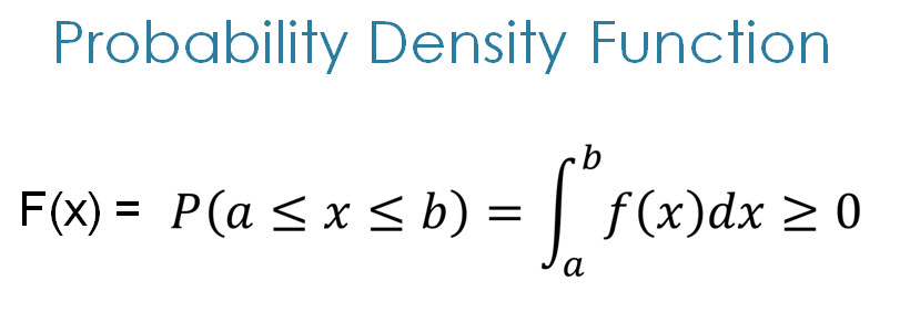
The formula for PDF.
Probability Mass Function (PMF)
It is a statistical term that describes the probability distribution of a discrete random variable.
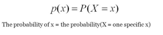
The formula for PMF.
Cumulative Distribution Function (CDF)
It is another method to describe the distribution of a random variable (either continuous or discrete).
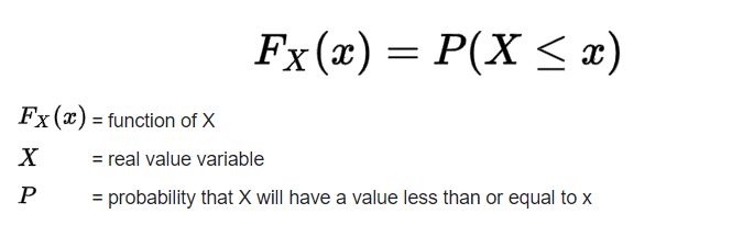
The formula for CDF.
Discrete distributions
Let us start with the easiest one – Uniform distribution.
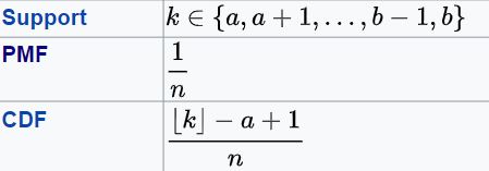
Discrete Uniform distribution (U)
It is denoted as X ~ U (a, b). And is read as X is a discrete random variable that follows uniform distribution ranging from a to b.
Uniform distribution is when all the possible events are equally likely. For example, consider an experiment of rolling a dice. We have six possible events X = {1, 2, 3, 4, 5, 6} each having a probability of P(X) = 1/6.
The PMF graph of the above experiment is:

The formula for PMF, CDF of Uniform distribution function are:
The Mean and Variance of Uniform distribution are:
Mean = (a+b)/2
Variance = (n2-1)/12
Binomial distribution (B):
It is denoted as X ~ B(n, p). And is read as X is a discrete random variable that follows Binomial distribution with parameters n, p.
Where n is the no. of trials, and p is the success probability for each trial.
Binomial distribution is a discrete probability distribution of the number of successes in ‘n’ independent experiments sequence. The two outcomes of a Binomial trial could be Success/Failure, Pass/Fail/, Win/Lose, etc.
Generally, the outcome success is denoted as 1, and the probability associated with it is p.
And Failure is denoted as 0, and the probability associate with it is q = 1-p.
The formula for PMF, CDF of Binomial distribution are:
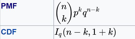
K in the above formula is the number of successes.
The mean and variance of a binomial distribution are given as:
Mean = np
Variance = npq
Now consider, we ran a Binomial experiment 10 times, and the probability of success = 0.25. Below are how PMF, CDF looks.
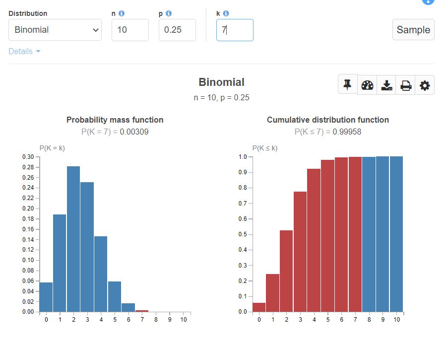
Image by Author
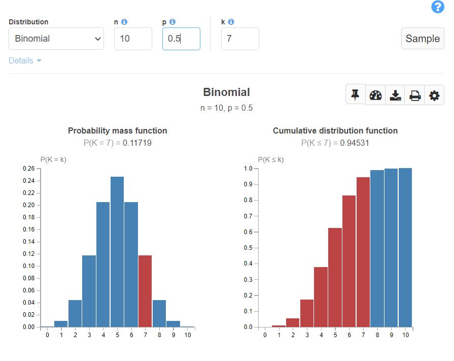
PMF, CDF for a Binomial experiment with Probability of success = Probability of failure look like below.
Bernoulli distribution (Bern):
It is denoted as X ~ Bern(p). And is read as X is a discrete random variable that follows Bernoulli distribution with parameter p.
Where p is the probability of the success.
Bernoulli can be represented as a Binomial experiment with a single trial.
X ~ Bern(p) —-> X ~ B(1, p)
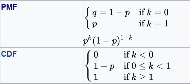
The formula for PMF, CDF of Bernoulli distribution is:
The Mean and Variance of Bernoulli distribution are given as:
Mean = p
Variance = p(1-p) = pq
Example: Consider an example of tossing a fair. The two possible outcomes are Heads, Tails. The probability (p) associated with each of them is 1/2.
If we take an unfair coin, the probability associated with each of them need not be 1/2. Heads can have a probability of p = 0.8, then the probability of tail q = 1-p = 1-0.8 = 0.2
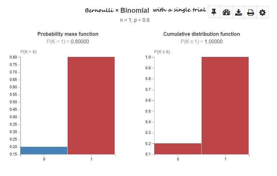
Bernoulli’s event suggests which outcome can be expected for a single trial. Whereas, a Binomial event suggests the no. of times a specific outcome can be expected.
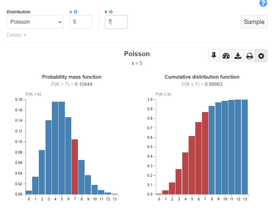
Poisson Distribution (Po):
It is denoted as X ~ Po(λ). And is read as X is a discrete random variable that follows Poisson Distribution with parameter λ.
Where λ is the expected rate of occurrences.
Poisson Distribution is a discrete probability distribution function that expresses the probability of a given number of events occurring in a fixed time interval.
Examples:
- The number of diners at a restaurant on a given day.
- Calls per hour at a call centre.
The formula for PMF, CDF of poison distribution are:
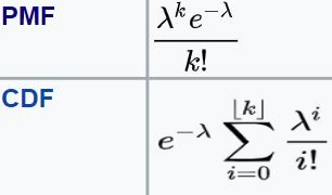
The Mean and Variance of Poisson distribution are given as:
Mean = Variance = λ
A Poisson distribution with λ = 5 look like below
Continuous Distributions
Normal or Gaussian Distribution (N)
It is denoted as X ~ N (μ, σ2). And is read as X is a continuous random variable that follows a Normal distribution with parameters μ, σ2.
Where μ is the mean, and σ2 is the variance. Mean, Variance together talks about shape statistics.
A normal distribution is a continuous distribution that describes the probability of a continuous random variable that takes real values.
Examples: Heights of people, exam scores of students, IQ Scores, etc follows Normal distribution.
Properties of Normal distribution:
- The random variable takes values from -∞ to +∞
- The probability associate with any single value is Zero.
- looks like a bell curve and is symmetric about x=μ. 50% of data lies on the left-hand side and 50% of the data lies on the right-hand side.
- The area under the curve (AUC) = 1
- All the measures of central tendency coincide i.e., mean = median = mode
A normal distribution with different means, standard deviations look like below:
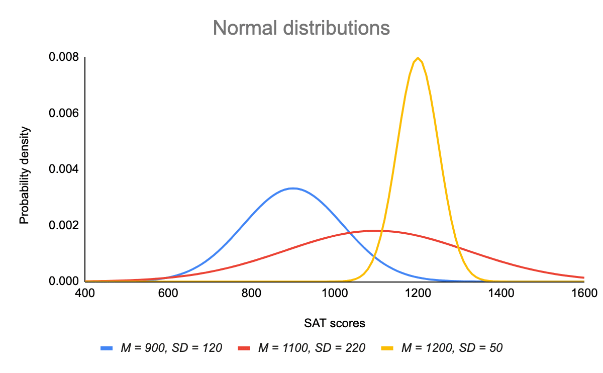
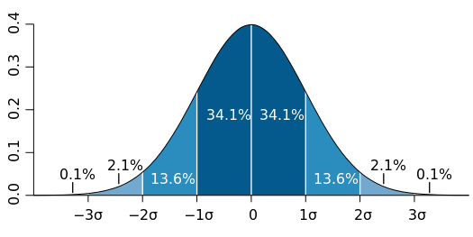
Normal distribution follows the 68-95-99.7 rule. This rule is also known as the empirical rule. According to it, 68% of data lies in the first standard deviation range, 95% of data lies in the second standard deviation range, and 99.7% of data lies in the third standard deviation range.

The formula for PDF, CDF of the normal distribution are:
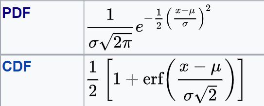
The Mean and Variance of a Normal distribution are given as:
Mean = μ
Variance = σ2
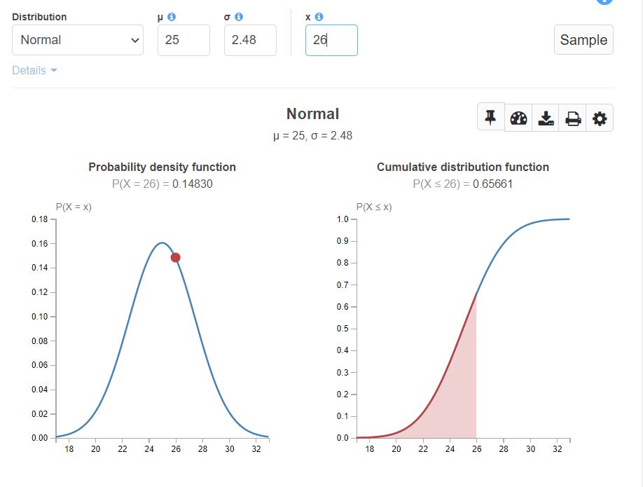
Let’s assume we have a height distribution with mean = 25, standard deviation = 2.48. Below is how the graph looks like.
Standard Normal Distribution or SND:
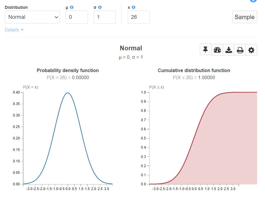
It is denoted as Z ~ N(0, 1). And is read as X is a continuous random variable that follows Normal distribution with mean 0 and variance 1.
It is a transformation of Normal distribution in such a way that Mean = 0, and standard deviation 1.
Transformation is a way in which we alter every element of distribution to get a new distribution with similar characteristics.
All the properties of a Normal distribution will be satisfied by a Standard Normal distribution.
And in addition, there exists a table that summarizes the most commonly used values of a CDF of s Standard Normal Distribution. This table is known as a Z-score table.
The formula for standardisation is Z = (X-μ)/σ
The formula for PDF, CDF of Standard Normal distribution are given as:
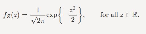
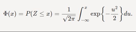
The Mean and Variance of Standard Normal distribution are:
Mean = 0
Variance = 1
Normal distribution with mean 0 and variance 1 (SND) looks like below:
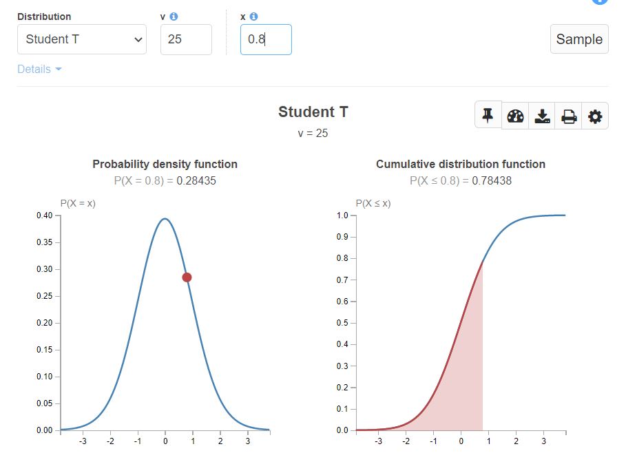
Student’s T distribution or t-distribution (t)
It is denoted as X ~ t(k). And is read as X is a continuous random variable that follows Student’s T distribution with parameter k.
where k is the degrees of freedom. If the sample size is n, then k = n-1.
Student’s T distribution is a small sample size approximation of a normal distribution. As the degrees of freedom increase, t distribution tends to become Standard Normal distribution.
The formula for PDF, CDF of t-distribution are:
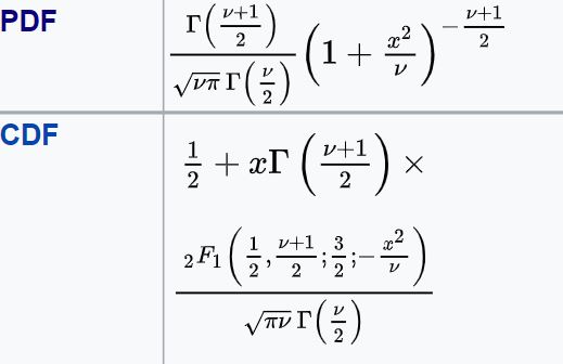
(v in above formulae is degrees of freedom)
t-distribution can be used in Hypothesis testing (to test if there is any significant difference between two sample means), calculating confidence intervals with population standard deviation is unknown.
Like standard normal distribution, t-distribution also has a table of its own. This table is known as the t-table.
The mean and variance of Student’s T distribution are:
Mean = 0
variance = k/(k-2)
A student’s t-distribution with degrees of freedom = 25 looks like below:
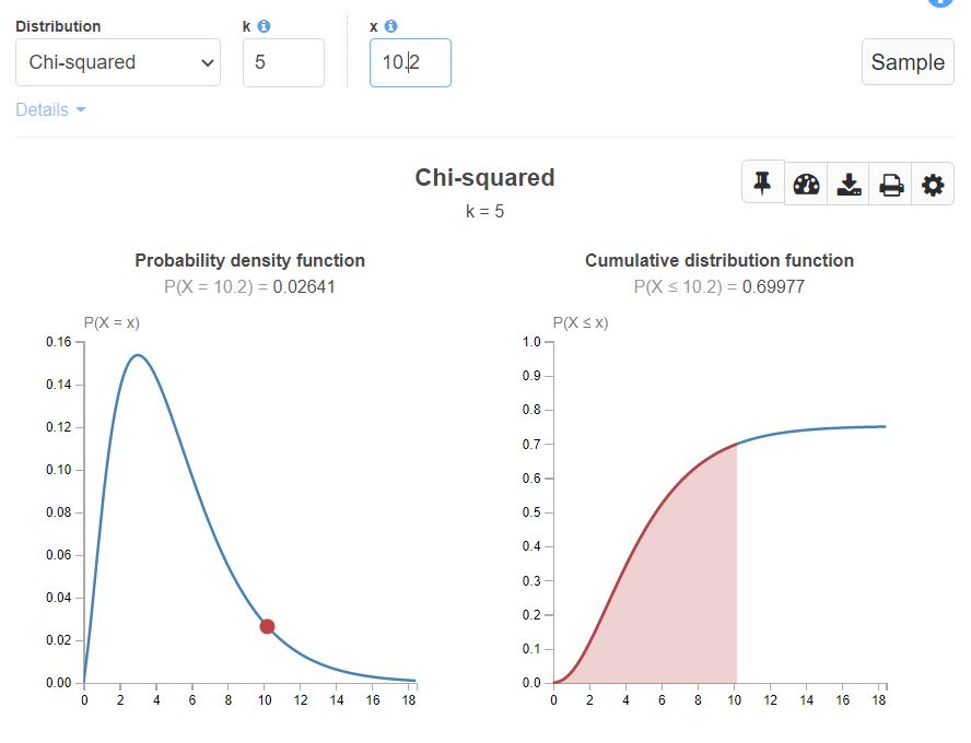
Chi-Square distribution
It is denoted as X~χ2(k). And is read as X is a continuous random variable that follows Chi-Square distribution with k degrees of freedom.
It is used in Hypothesis testing, computing confidence intervals, and for the goodness of fit.
It is a transformation of t-distribution. Finding the t-distribution to the power of 2 gives Chi-Square distribution and finding the square root of Chi-Square of distribution gives us t-distribution.
Chi-Square distribution has a chi-square table.
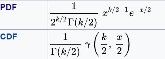
The formula for PDF, CDF of Chi-square distribution are:
The mean and variance of Chi-square distribution are:
Mean = k
Variance = 2k
A Chi-square distribution with degrees of freedom = 5 looks like below.
Conclusion
In summary, Probability Distribution Functions (PDFs) and their formulas and Distribution Functions are key for understanding different data types. Explore Discrete Uniform, Binomial, Bernoulli, Poisson, and Continuous distributions to gain insights for effective data analysis and decision-making in various scenarios.
I hope this article is informative. Feel free to share it with your study buddies.
The media shown in this article are not owned by Analytics Vidhya and are used at the Author’s discretion.
Frequently Asked Questions?
Q1. What is probability distribution functions?
A. Probability distribution functions describe the probabilities of possible outcomes in a random phenomenon. They assign probabilities to various events or values that a random variable can take.
Q2. What is the state probability distribution function?
A. The state probability distribution function describes the probabilities of a system being in different states or conditions. It’s commonly used in fields like physics, chemistry, and engineering to model the behavior of systems in different states.
Q3. What is the expression for the probability distribution function?
A. The expression for the probability distribution function varies depending on the specific distribution being considered. For example, for a continuous distribution, it might be expressed as a probability density function (PDF), while for a discrete distribution, it might be expressed as a probability mass function (PMF).
Q4. What is the probability distribution function also called?
A. The probability distribution function is also commonly referred to as the probability density function (PDF) for continuous distributions or the probability mass function (PMF) for discrete distributions.
blogathondata scienceDistribution functionfollowing is a discrete probability distribution functionprobability distributionproperties of probability distribution functionstatistics
Harika Bonthu
09 Apr, 2024


