Time-series Forecasting -Complete Tutorial | Part-1
This article was published as a part of the Data Science Blogathon
Introduction
A time series is a sequence of observations recorded over a certain period of time. A simple example of time-series forecasting is how we come across different temperature changes day by day or in a month. The tutorial will give you a complete sort of understanding of what is time-series data, what methods are used to forecast time series, and what makes time series data so special a complex topic in the field of data science.

Table of contents
What is Time-Series Forecasting
Time-series forecasting in simple words means to forecast or to predict the future value(eg-stock price) over a period of time. There are different approaches to predict the value, consider an example there is a company XYZ records the website traffic in each hour and now wants to forecast the total traffic of the coming hour. If I ask you what will your approach to forecasting the upcoming hour traffic?
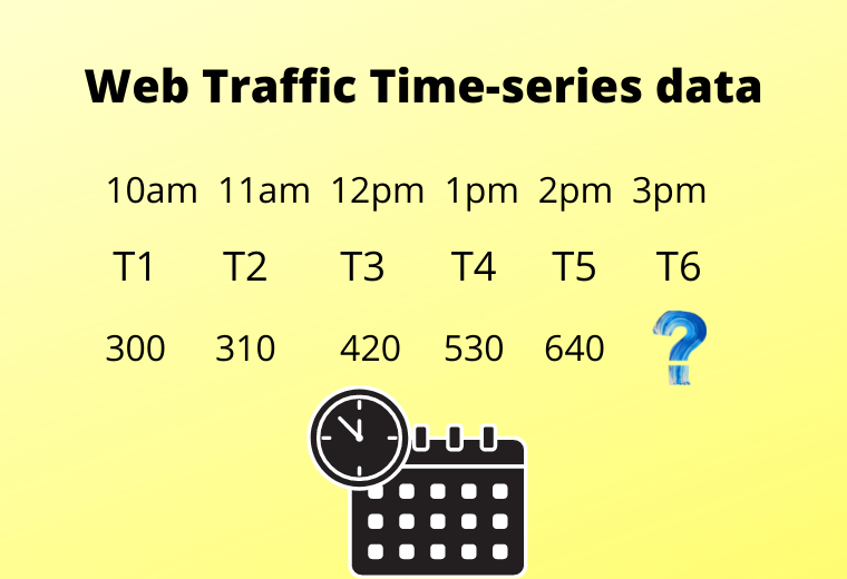
A different person can have a different perspective like one can say find the mean of all observations, one can have like take mean of recent two observations, one can say like give more weightage to current observation and less to past, or one can say use interpolation. There are different methods to forecast the values.
while Forecasting time series values, 3 important terms need to be taken care of and the main task of time series forecasting is to forecast these three terms.
1) Seasonality
Seasonality is a simple term that means while predicting a time series data there are some months in a particular domain where the output value is at a peak as compared to other months. for example if you observe the data of tours and travels companies of past 3 years then you can see that in November and December the distribution will be very high due to holiday season and festival season. So while forecasting time series data we need to capture this seasonality.
2) Trend
The trend is also one of the important factors which describe that there is certainly increasing or decreasing trend time series, which actually means the value of organization or sales over a period of time and seasonality is increasing or decreasing.
3) Unexpected Events
Unexpected events mean some dynamic changes occur in an organization, or in the market which cannot be captured. for example a current pandemic we are suffering from, and if you observe the Sensex or nifty chart there is a huge decrease in stock price which is an unexpected event that occurs in the surrounding.
Methods and algorithms are using which we can capture seasonality and trend But the unexpected event occurs dynamically so capturing this becomes very difficult.
Rolling Statistics and Stationarity in Time-series
A stationary time series is a data that has a constant mean and constant variance. If I take a mean of T1 and T2 and compare it with the mean of T4 and T5 then is it the same, and if different, how much difference is there? So, constant mean means this difference should be less, and the same with variance.
If the time series is not stationary, we have to make it stationary and then proceed with modelling. Rolling statistics is help us in making time series stationary. so basically rolling statistics calculates moving average. To calculate the moving average we need to define the window size which is basically how much past values to be considered.
For example, if we take the window as 2 then to calculate a moving average in the above example then, at point T1 it will be blank, at point T2 it will be the mean of T1 and T2, at point T3 mean of T3 and T2, and so on. And after calculating all moving averages if you plot the line above actual values and calculated moving averages then you can see that the plot will be smooth.
This is one method of making time series stationary, there are other methods also which we are going to study as Exponential smoothing.
Additive and Multiplicative Time series
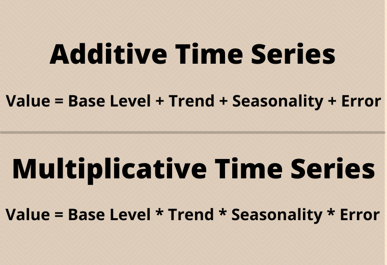
In the real world, we meet with different kinds of time series data. For this, we must know the concepts of Exponential smoothing and for this first, we need to study types of time series data as additive and multiplicative. As we studied there are 3 components we need to capture as Trend(T), seasonality(S), and Irregularity(I).
Additive time series is a combination(addition) of trend, seasonality, and Irregularity while multiplicative time series is the multiplication of these three terms.
Time series Exponential Smoothing
Exponential smoothing calculates the moving average by considering more past values and give them weightage as per their occurrence, as recent observation gets more weightage compared to past observation so that the prediction is accurate. hence the formula of exponential smoothing can be defined as.
yT = α * XT + α(1−α) * yT−1
Alpha is a hyperparameter that defines the weightage to give. This is known as simple exponential smoothing, But we need to capture trend and seasonality components so there is double exponential smoothing which is used to capture the trend components. only a little bit of modification in the above equation is there.
Yt = α * Xt + (1-α) (yt-1 + bt-1) #trend component
where, bt = beta * (Yt – Yt-1) + (1-beta) * bt-1
hence here we are taking 2 past observations and what was in the previous cycle, which means we are taking two consecutive sequences, so this equation will give us the trend factor.
If we need to capture trend and seasonality for both components then it is known as triple exponential smoothing which adds another layer on top of trend exponential smoothing where we need to calculate trend and seasonality for both.
Y = alpha * (Xt / Ct-1) + (1 – alpha)*(Y t-1 + bt-1)
where, ct = gamma * (xt/yt) + (1-alpha) * ct-alpha
here we are capturing trends as well as seasonality. Using smoothing we will be able to decompose our time series data and our time-series data will become easy to work with because in real-world scenarios working with time series is a complex task so you have to adopt such methods to make the process smooth.
Practicals with Time series forecasting
It’s time to make our hands dirty by implementing the concepts we have learned so far till now from start. we will implement Moving average, exponential smoothing methods and compare them with an original distribution of data.
Exponential smoothing practicals
The dataset we are using is electricity consumption time series data and you can easily find it on Kaggle from here.
step-1) Load the data first
Python Code:

Step-2) Moving Average method
we have seen how to calculate moving average using a window, same applies to our dataset and we will get rolling statistics and find its mean. after the mean, if we plot the graph then you can see the difference in smoothing of a graph as the original.
rollingseries = df[1:50].rolling(window=5)
rollingmean = rollingseries.mean() #we can compute any statistical measure
#print(rollingmean.head(10))
rollingmean.plot(color="red")
plt.show()
Step-3) Simple Exponential Smoothing
Now as we have seen in simple exponential smoothing has a parameter known as alpha which defines how much weightage we want to give to recent observation. we will fit 2 models, one with high value and one with less value of alpha, and compare both.
data = df[1:50]
fit1 = SimpleExpSmoothing(data).fit(smoothing_level=0.2, optimized=False)
fit2 = SimpleExpSmoothing(data).fit(smoothing_level=0.8, optimized=False)
plt.figure(figsize=(18, 8))
plt.plot(df[1:50], marker='o', color="black")
plt.plot(fit1.fittedvalues, marker="o", color="b")
plt.plot(fit2.fittedvalues, marker="o", color="r")
plt.xticks(rotation="vertical")
plt.show()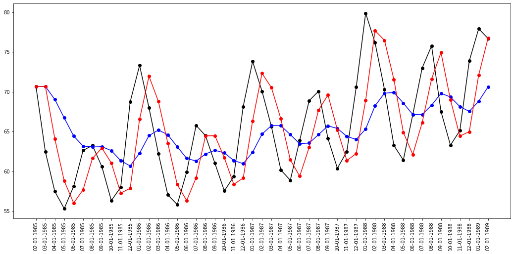
Step-4) Holt method for exponential smoothing
Hot’s method is a popular method for exponential smoothing and is also known as Linear exponential smoothing. It forecast the data with the trend. It works on three separate equations that work together to generate the final forecast. let us apply this to our data and experience the changes. In the first fit, we are assuming that there is a linear trend in data, and in the second fitting, we are having exponential smoothing.
fit1 = Holt(data).fit()  #linear trend
fit2 = Holt(data, exponential=True).fit()  #exponential trend
plt.plot(data, marker='o', color='black')
plt.plot(fit1.fittedvalues, marker='o', color='b')
plt.plot(fit2.fittedvalues, marker='o', color='r')
plt.xticks(rotation="vertical")
plt.show()
You can observe that linear trend means blue plot does not fit fine, and following the original plot whereas red plot is an exponential smoothing plot. This is a simple smoothing with the holt method, we also add parameters like alpha, trend component, seasonality component.
Decomposition and stationarity check practicals
Now we will work and check which type of time series data we have, whether it is additive or multiplicative. We will use a different dataset from above and it is known as drug sales data which you can download from here.
Step-1) Load dataset
If you observe the above plot then we can see the upward trend in the data, but we cannot see any kind of special seasonality.
from statsmodels.tsa.seasonal import seasonal_decompose
from dateutil.parser import parse
import pandas as pd
DrugSalesData = pd.read_csv('TimeSeries.csv', parse_dates=['Date'], index_col='Date')
DrugSalesData.reset_index(inplace=True)
import matplotlib.pyplot as plt
plt.rcParams.update({'figure.figsize': (10,6)})
plt.plot(DrugSalesData['Value'])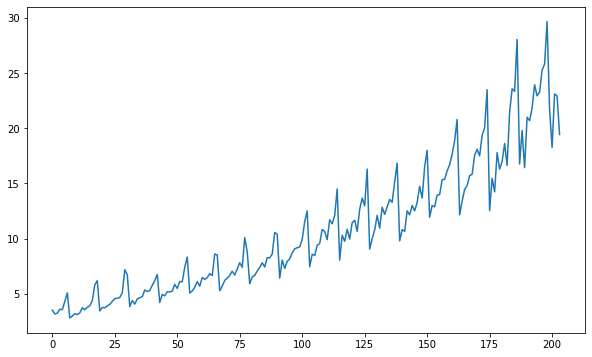
Step-2) Decomposition of time-series data
Now we will decompose time series data into multiplicative and additive and visualize the seasonal and trend components that they have extracted.
# Additive Decomposition
add_result = seasonal_decompose(DrugSalesData['Value'], model='additive',period=1)
# Multiplicative Decomposition
mul_result = seasonal_decompose(DrugSalesData['Value'], model='multiplicative',period=1)
We imported the seasonal decompose function from the stats model and pass both the model as multiplicative and additive. Now let us visualize the result of each model one by one. first plot the results of the Additive time series.
add_result.plot().suptitle('nAdditive Decompose', fontsize=12)
plt.show()
If you observe the plots you will get 4 plots, two for trend, one for seasonality, and one for residual. We can see that trend is of course there using both time methods and seasonality is zero.
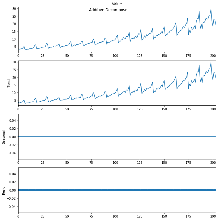
Now we also want to see the actual value of trend and seasonality, how much it has been calculated. so we will prepare the dataframe of four columns which will have a value for each plot. let us make of additive, and you can try will multiplicative in the same way.
new_df_add = pd.concat([add_result.seasonal, add_result.trend, add_result.resid, add_result.observed], axis=1)
new_df_add.columns = ['seasoanilty', 'trend', 'residual', 'actual_values']
new_df_add.head()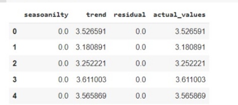
Step-3) ADfuller test for stationary
Stationary is constantly mean and constant variance. Adfuller is a simple test which tells that if the time series is stationary which is a kind of hypothesis testing. The Null hypothesis is time series are non-stationary. If the p-value is less than 5 percent then reject the NULL hypothesis else accept the NULL hypothesis.
from statsmodels.tsa.stattools import adfuller
adfuller_result = adfuller(DrugSalesData.Value.values, autolag='AIC')
print(f'ADF Statistic: {adfuller_result[0]}')
print(f'p-value: {adfuller_result[1]}')
for key, value in adfuller_result[4].items():
    print('Critial Values:')
    print(f'   {key}, {value}')
P-value is greater than 5 per cent, which means we cannot build a model on Non-stationary data so we have to make the time series stationary. Now to make time-series stationary there are different methods like autoregression with ACF, PACF, etc which we will cover in the second part of this article.
End Notes
We have seen what is time-series data, what makes time-series analysis a special and complex task in Machine learning. We also perform practicals on how to start working with time series data and how to perform various analyses and drive inferences from it. In the upcoming part, we will discuss various methods to make time-series stationary and we will also discuss various time-series Forecasting classical models like ARIMA, SARIMA, etc.
I hope it was easy to follow till the end, I know it’s a little complex to handle time-series data But after having a look through this article you got some sort of understanding and confidence that you can handle time-series data. If you have any queries, please post them in the comment section below.
Frequently Asked Questions
Five time- series forecasting methods:
Moving Average
Exponential Smoothing
ARIMA (AutoRegressive Integrated Moving Average)
Prophet
Machine Learning Models
Time-series forecasting simple:
Time series forecast is a way to predict future values based on past data. Think of it like looking at a graph of temperature over several days and guessing what the temperature might be tomorrow or next week based on the patterns you see in the graph.


This article is really helpful. Very easy to understand. Great work. Can you please share part 2 ?
Hi I loved this article its concise and informative can you help me find part 2 of this tutorial
I think that there is a seasonality in the data. The mean changes over time and is the upward trend. The regular pattern is the cycles or seasonality. is the upwards curve and the seasonality is the spikes. Try a period of 12.
This is really awesome fr a beginner to learn about time series basics