Understanding the Basics Of Artificial Neural Network

This article was published as a part of the Data Science Blogathon

INTRODUCTION

In this article, I will explain to you the basics of neural networks and their code. Nowadays many students just learn how to code for neural networks without understanding the core concepts behind it and how it internally works. First,  Understand what is Neural Networks?

What is Neural Network?

Neural Network is a series of algorithms that are trying to mimic the human brain and find the relationship between the sets of data. It is being used in various use-cases like in regression, classification, Image Recognition and many more.

As we have talked above that neural networks tries to mimic the human brain then there might be the difference as well as the similarity between them. Let us talk in brief about it.

Some major differences between them are biological neural network does parallel processing whereas the Artificial neural network does series processing also in the former one processing is slower (in millisecond) while in the latter one processing is faster (in a nanosecond).

Architecture Of ANN

A neural network has many layers and each layer performs a specific function, and as the complexity of the model increases, the number of layers also increases that why it is known as the multi-layer perceptron.

The purest form of a neural network has three layers input layer, the hidden layer, and the output layer. The input layer picks up the input signals and transfers them to the next layer and finally, the output layer gives the final prediction and these neural networks have to be trained with some training data as well like machine learning algorithms before providing a particular problem. Now, let’s understand more about perceptron.

About Perceptron

As discussed above multi-layered perceptron these are basically the hidden or the dense layers. They are made up of many neurons and neurons are the primary unit that works together to form perceptron. In simple words, as you can see in the above picture each circle represents neurons and a vertical combination of neurons represents perceptrons which is basically a dense layer.

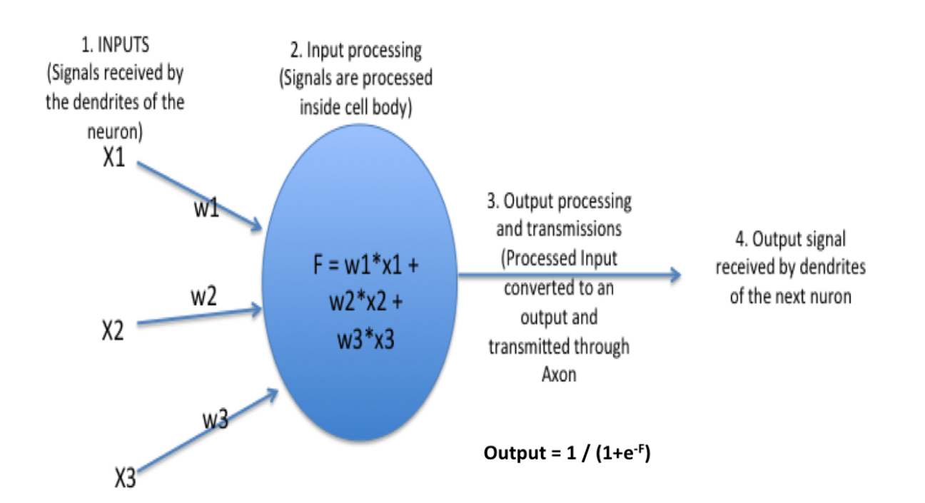
Now in the above picture, you can see each neuron’s detailed view. Here, each neurons have some weights (in above picture w1, w2, w3) and biases and based on this computations are done as, combination = bias + weights * input (F = w1*x1 + w2*x2 + w3*x3) and finally activation function is applied output = activation(combination) in above picture activation is sigmoid represented by      1/(1 + e^-F). There are some other activation functions as well like ReLU, Leaky ReLU, tanh, and many more.

Working Of ANN

At First, information is feed into the input layer which then transfers it to the hidden layers, and interconnection between these two layers assign weights to each input randomly at the initial point. and then bias is added to each input neuron and after this, the weighted sum which is a combination of weights and bias is passed through the activation function. Activation Function has the responsibility of which node to fire for feature extraction and finally output is calculated. This whole process is known as Foreward Propagation. After getting the output model to compare it with the original output and the error is known and finally, weights are updated in backward propagation to reduce the error and this process continues for a certain number of epochs (iteration). Finally, model weights get updated and prediction is done.

Advantages

1. ANN has the ability to learn and model non-linear and complex relationships as many relationships between input and output are non-linear.
2. After training, ANN can infer unseen relationships from unseen data, and hence it is generalized.
3. Unlike many machine learning models, ANN does not have restrictions on datasets like data should be Gaussian distributed or nay other distribution.

Applications

There are many applications of ANN. Some of them are :

1. Image Preprocessing and Character Recognition.
2. Forecasting.
3. Credit rating.
4. Fraud Detection.
5. Portfolio Management.

CODING PART

Now let’s code and understand the concepts using it.

1. Understanding and Loading the datasets

First Import Libraries like NumPy, pandas, and also import classes named sequential and dense from Keras library.

import numpy as np
import pandas as pd
from keras.models import Sequential
from keras.layers import Dense

Now here I am going to use the Pima Indians onset of diabetes dataset which is a standard machine learning dataset from the UCI Machine Learning repository and the link can be found below. This dataset tells about the patient medical record and whether they had an onset of diabetes within five years also it is a binary classification problem.

You can download the datasets from here:

Datasets

Now import the dataset using pandas and then let us understand more about the datasets and then split the datasets into dependent and independent variables.

#import numpy as np
import pandas as pd
#from keras.models import Sequential
#from keras.layers import Dense

dataset = pd.read_csv('raw.csv')
print(dataset.head())
X = dataset.iloc[:,0:8]
y = dataset.iloc[:,8]
print(X)
print(y)

2. Defining the Keras Model

Models in Keras are defined as a sequence of layers in which each layer is added one after another. The input should contain input features and is specified when creating the first layer with the input_dims argument. Here inputs_dims will be 8.

Now a question arises that how can we decide the number of layers and number of neurons in each layer?

It is quite difficult to know how many layers we should use. Generally for this Keras tuner is used, which takes a range of layers, a range of neurons, and some activation functions. and then by permutation and combination, it tries to find which is best suited. But one disadvantage of this is it takes lots of time. You can refer to the documentation of it Keras Tuner for more details. 

In this example, a fully connected network with a three-layer is used which is defined using the Dense Class. The first argument takes the number of neurons in that layer and, and the activation argument takes the activation function as an input. Here ReLU is used as an activation function in the first two layers and sigmoid in the last layer as it is a binary classification problem.

model = Sequential()
model.add(Dense(12, input_dim=8, activation='relu'))
model.add(Dense(8, activation='relu'))
model.add(Dense(1, activation='sigmoid'))

3. Compile Keras Model

While compiling we must specify the loss function to calculate the errors, the optimizer for updating the weights and any metrics.

In this case, we will use “binary_crossentropy“ as the loss argument as it is a binary classification problem.

Here we will take optimizer as “adam“ as it automatically tunes itself and gives good results in a wide range of problems and finally we will collect and report the classification accuracy through metrics argument.

model.compile(loss='binary_crossentropy', optimizer='adam', metrics=['accuracy'])

4. Fitting The Keras Model.

Now we will fit our model on the loaded data by calling the fit() function on the model.

The training process will run for a fixed number of iterations through the dataset which is specified using the epochs argument. The number of dataset rows should be and are updated within each epoch, and set using the batch_size argument.

Here, We will run for 150 epochs and a batch size of 10.

model.fit(X, y, epochs=150, batch_size=10)

5. Evaluate Keras Model

The evaluation of the model on the dataset can be done using the evaluate() function. It takes two arguments i.e, input and output. It will generate a prediction for each input and output pair and collect scores, including the average loss and any metrics such as accuracy.

The evaluate() function will return a list with two values first one is the loss of the model and the second will be the accuracy of the model on the dataset. We are only interested in reporting the accuracy and hence we ignored the loss value.

_, accuracy = model.evaluate(X, y)
print('Accuracy: %.2f' % (accuracy*100))

6. Make Predictions

Prediction can be done by calling the predict() function on the model. Here sigmoid activation function is used on the output layer, so the predictions will be a probability in the range between 0 and 1.

predictions = model.predict(X)
rounded = [round(x[0]) for x in predictions]

Final Code Summary

Here we have learned how to create your first neural network model using the powerful Keras Python library for deep learning.

There are six main steps in using Keras to create a neural network or deep learning model that are loading the data, defining the neural network in Keras after that compiling, evaluating, and finally making the predictions with the model.

CONCLUSION

In this article, we have understood the basic concepts of Artificial neural networks and their code. In the coding part, we have used the Pima Indians’ onset of diabetes dataset. here we have understood in detail all six main steps to create neural networks. Apart from this many things have not been covered in the blogs and below I have provided the links of other blogs from which you can refer the topics.

1. Different types of cost functions and their applications.
2. About Gradient Descent.
3. Keras Documentation