This article was published as a part of the Data Science Blogathon
We have learned about the Artificial Neural network and its application in the last few articles. This blog will be all about another Deep Learning model which is the Convolutional Neural Network. As always this will be a beginner’s guide and will be written in such as matter that a starter in the Data Science field will be able to understand the concept, so keep on reading 🙂
3. Practical Implementation of CNN on a dataset
Convolutional Neural Network is a Deep Learning algorithm specially designed for working with Images and videos. It takes images as inputs, extracts and learns the features of the image, and classifies them based on the learned features.
This algorithm is inspired by the working of a part of the human brain which is the Visual Cortex. The visual Cortex is a part of the human brain which is responsible for processing visual information from the outside world. It has various layers and each layer has its own functioning i.e each layer extracts some information from the image or any visual and at last all the information received from each layer is combined and the image/visual is interpreted or classified.
Similarly, CNN has various filters, and each filter extracts some information from the image such as edges, different kinds of shapes (vertical, horizontal, round), and then all of these are combined to identify the image.
Now, the question here can be: Why can’t we use Artificial Neural Networks for the same purpose? This is because there are some disadvantages with ANN:
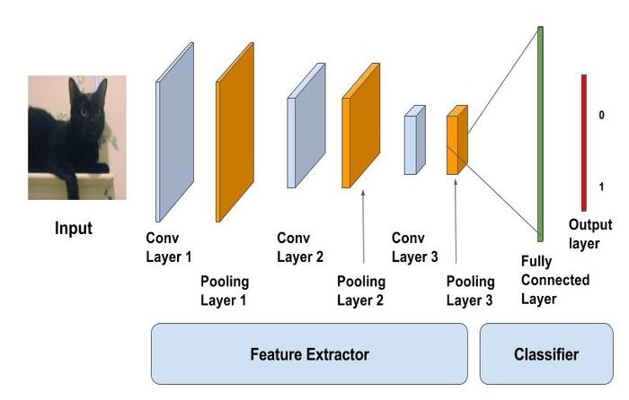
The CNN model works in two steps: feature extraction and Classification
Feature Extraction is a phase where various filters and layers are applied to the images to extract the information and features out of it and once it’s done it is passed on to the next phase i.e Classification where they are classified based on the target variable of the problem.
A typical CNN model looks like this:

Source: https://learnopencv.com/image-classification-using-convolutional-neural-networks-in-keras/
Let’s learn about each layer in detail.
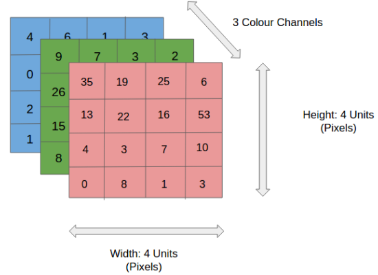
As the name says, it’s our input image and can be Grayscale or RGB. Every image is made up of pixels that range from 0 to 255. We need to normalize them i.e convert the range between 0 to 1 before passing it to the model.
Below is the example of an input image of size 4*4 and has 3 channels i.e RGB and pixel values.

The convolution layer is the layer where the filter is applied to our input image to extract or detect its features. A filter is applied to the image multiple times and creates a feature map which helps in classifying the input image. Let’s understand this with the help of an example. For simplicity, we will take a 2D input image with normalized pixels.
.png)
In the above figure, we have an input image of size 6*6 and applied a filter of 3*3 on it to detect some features. In this example, we have applied only one filter but in practice, many such filters are applied to extract information from the image.
The result of applying the filter to the image is that we get a Feature Map of 4*4 which has some information about the input image. Many such feature maps are generated in practical applications.
Let’s get into some maths behind getting the feature map in the above image.
.png)
As presented in the above figure, in the first step the filter is applied to the green highlighted part of the image, and the pixel values of the image are multiplied with the values of the filter (as shown in the figure using lines) and then summed up to get the final value.
In the next step, the filter is shifted by one column as shown in the below figure. This jump to the next column or row is known as stride and in this example, we are taking a stride of 1 which means we are shifting by one column.
.png)
Similarly, the filter passes over the entire image and we get our final Feature Map. Once we get the feature map, an activation function is applied to it for introducing nonlinearity.
A point to note here is that the Feature map we get is smaller than the size of our image. As we increase the value of stride the size of the feature map decreases.
.png)
The pooling layer is applied after the Convolutional layer and is used to reduce the dimensions of the feature map which helps in preserving the important information or features of the input image and reduces the computation time.
Using pooling, a lower resolution version of input is created that still contains the large or important elements of the input image.
The most common types of Pooling are Max Pooling and Average Pooling. The below figure shows how Max Pooling works. Using the Feature map which we got from the above example to apply Pooling. Here we are using a Pooling layer of size 2*2 with a stride of 2.
The maximum value from each highlighted area is taken and a new version of the input image is obtained which is of size 2*2 so after applying Pooling the dimension of the feature map has reduced.
.png)
Till now we have performed the Feature Extraction steps, now comes the Classification part. The Fully connected layer (as we have in ANN) is used for classifying the input image into a label. This layer connects the information extracted from the previous steps (i.e Convolution layer and Pooling layers) to the output layer and eventually classifies the input into the desired label.
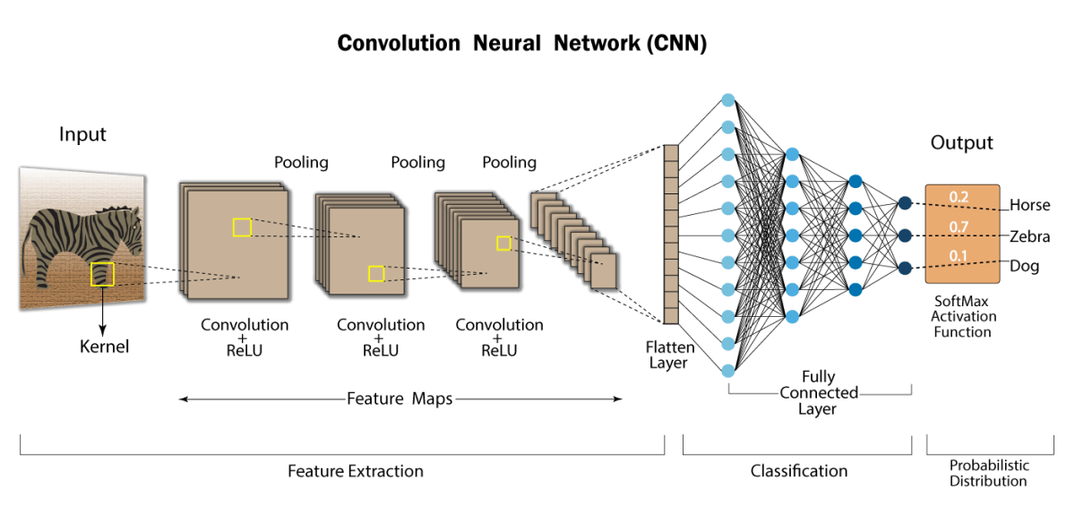
The complete process of a CNN model can be seen in the below image.

Source: https://developersbreach.com/convolution-neural-network-deep-learning/
We will be using the Mnist Digit classification dataset which we used in the last blog of Practical Implementation of ANN. Please refer to that first for a better understanding of the application of CNN.
from tensorflow.keras.datasets import mnist
from tensorflow.keras.models import Sequential
from tensorflow.keras.layers import Conv2D
from tensorflow.keras.layers import MaxPool2D
from tensorflow.keras.layers import Flatten
from tensorflow.keras.layers import Dropout
from tensorflow.keras.layers import Dense
(X_train,y_train) , (X_test,y_test)=mnist.load_data()
X_train = X_train.reshape((X_train.shape[0], X_train.shape[1], X_train.shape[2], 1))
X_test = X_test.reshape((X_test.shape[0],X_test.shape[1],X_test.shape[2],1))
print(X_train.shape)
print(X_test.shape)
X_train=X_train/255
X_test=X_test/255
model=Sequential()model=Sequential()
model.add(Conv2D(32,(3,3),activation=’relu’,input_shape=(28,28,1)))
model.add(MaxPool2D(2,2))
model.add(Flatten())
model.add(Dense(100,activation=’relu’))
model.add(Dense(10,activation=’softmax’))
model.compile(loss=’sparse_categorical_crossentropy’,optimizer=’adam’,metrics=[‘accuracy’])
model.fit(X_train,y_train,epochs=10)
Output:
.png)
#evaluting the model
model.evaluate(X_test,y_test)
.png)
A. A Convolutional Neural Network (CNN) is a type of deep neural network used for image recognition and classification tasks in machine learning. Python libraries like TensorFlow, Keras, PyTorch, and Caffe provide pre-built CNN architectures and tools for building and training them on specific datasets.
A. The four common types of Convolutional Neural Networks (CNNs) are LeNet, AlexNet, VGGNet, and ResNet. LeNet is the first CNN architecture used for handwritten digit recognition, while AlexNet, VGGNet, and ResNet are deep CNNs that achieved top performance on the ImageNet Large Scale Visual Recognition Challenge (ILSVRC).
A. TensorFlow is an open-source machine learning and artificial intelligence library developed by Google Brain Team. It is written in Python and provides high-level APIs like Keras, as well as low-level APIs, for building and training machine learning models. TensorFlow also offers tools for data preprocessing, visualization, and distributed computing.
We have covered some important elements of CNN in this blog while many are still left such as Padding, Data Augmentation, more details on Stride but as Deep learning is a deep and never-ending topic so I will try to discuss it in some future blogs. I hope you found this article helpful and worth your time investing on.
In the next few blogs, you can expect a detailed implementation of CNN with explanations and concepts like Data augmentation and Hyperparameter tuning.
I am Deepanshi Dhingra currently working as a Data Science Researcher, and possess knowledge of Analytics, Exploratory Data Analysis, Machine Learning, and Deep Learning. Feel free to content with me on LinkedIn for any feedback and suggestions.
The media shown in this article are not owned by Analytics Vidhya and are used at the Author’s discretion.
Lorem ipsum dolor sit amet, consectetur adipiscing elit,
this is an exquisite blog, thank you.
This is so useful. I am a beginner in this area. thank you so much
In a very simple way, explained CNN so beautifully and effectively. Excellent!