This article was published as a part of the Data Science Blogathon
Introduction
SciPy Toolkits or scikits are used widely for machine learning purposes. A scikit is a special toolkit used for specific purposes such as machine learning or image processing. Scikit-learn and Scikit-image are the two specialized packages that are used for these purposes. The package contains bundles of handy algorithms used to handle the processes involved in machine learning and image processing.
Scikits are extremely popular amongst programmers and software developers. The Scikit-learn can even be considered as one of the pillars of machine learning using Python. You can use this to create various models and prepare and evaluate data or even create post-model analysis.
Here, we are going to explore some essential knowledge needed to master scikit-learn and how it is useful for data scientists. This article contains the essence of the extremely useful package and its major salient features. Most of the illustrations used here are tagged from sources to help you understand the concepts better.
I know you’re eager to get started so let’s dive right in!
How Data is represented in scikit-learn
Scikit-learn can only be useful to you when you know the basics of what to use it for. A tabular dataset is what essentially is used for the data representation in this package. If you’re trying to design a supervised learning problem then this tabular dataset will have to contain both the x and y variables. However, if you’re trying to design an unsupervised learning problem then you need to provide only the x variables within the tabular dataset. The reason for this is that x variables are considered to be independent variables at a higher level. Meanwhile, the y variable is considered to be the dependent variable. Both x and y variables can be either qualitative or quantitative descriptions of samples of interest. Y variables are generally the target that predictive models are built to create. A sample dataset used in scikit-learn has been tagged below for a clearer understanding of the topic.

Source: https://unsplash.com/photos/1K6IQsQbizI
To understand this better let’s take an example. Suppose you are trying to build a predictive model that creates predictions of the possibility of individuals having/ not having a particular disease. Here, you required prediction that is whether an individual has/ doesn’t have the disease is held as the y variables which your model builds based on the x variable data. The x variable data in this case may be the results from clinical trials/tests that are used to diagnose the particular disease that you’re screening for.
Loading data using pandas
Mostly, datasets are practically stored as CSV files. These CSV files can be read using the Pandas library using the pd.read_csv() method. As a result of using this method, you’ll have the contents of the CSV file converted into the Pandas DataFrame. The illustration tagged below gives an example of this in process.
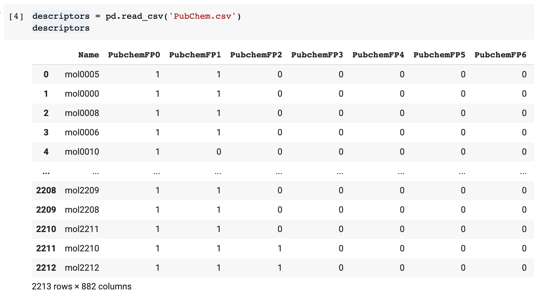
After you are done obtaining the Pandas DataFrame, you can use data processing techniques from the Pandas library to handle any dropped or missing data. You can also select a specific column or collection of columns and perform transformations or filter data according to various conditions.

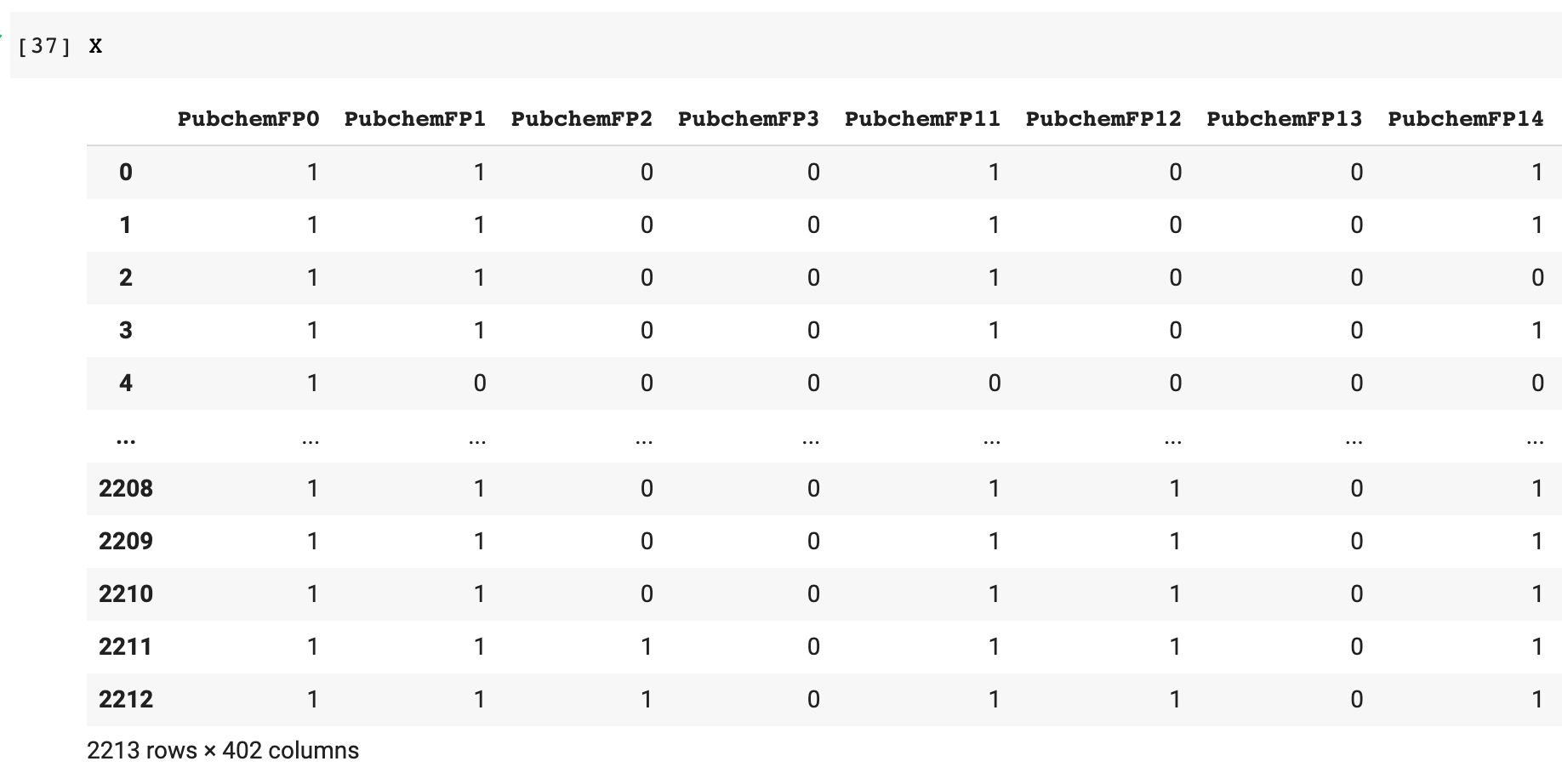
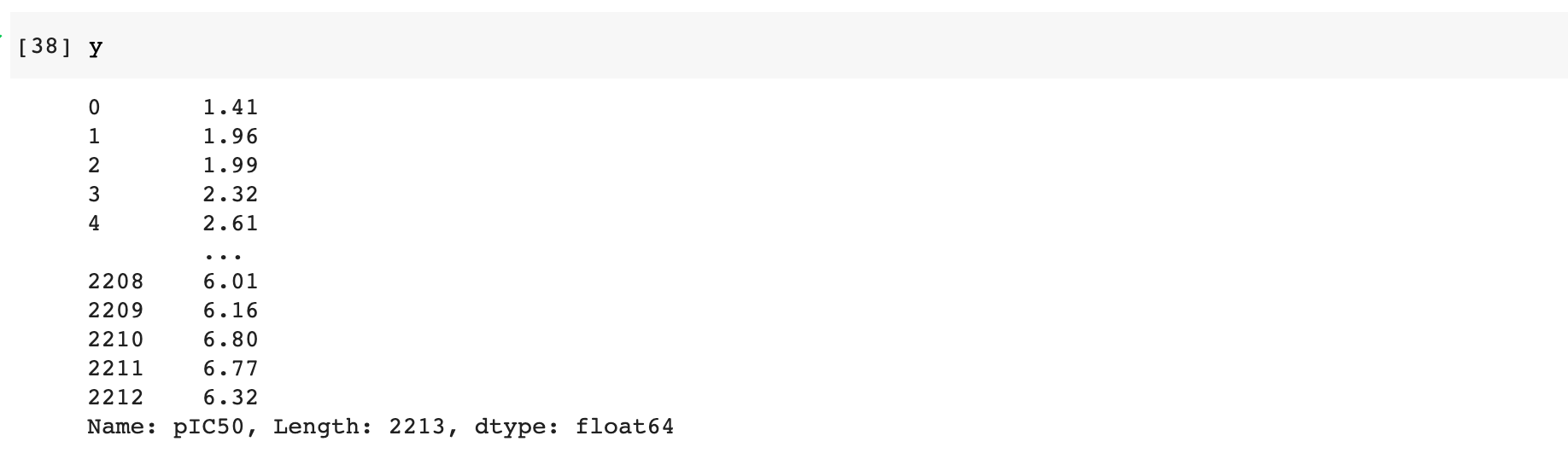
The above illustration shows how we can separate the DataFrame into x and y variables which will then be used for building your model.
Utility functions
The scikit-learn package has a lot of quick utility functions that assist its machine learning capabilities. Some of them have been tagged in this section. To become a master of the scikit-learn package you must have basic knowledge of these utility functions that can make your life easy.
1. To create a dataset
Machine learning workflows often require different datasets to arrive at the best model. You can use scikit-learn to create or devise artificial datasets that you can use with your model.
Code :
from sklearn.datasets import make_classification
X, Y = make_classification(n_samples=200, n_classes=2, n_features=10, n_redundant=0, random_state=1)
X,Y
Output :
(array([[-1.51107661,  0.60874908, -0.15323616, ..., -0.86482994,
         -0.20290111, -0.87142207],
        [ 1.44544531,  0.51896937,  0.64515265, ..., -1.04339961,
          0.04854689, -2.62101164],
        [ 0.37167029,  0.51350548, -1.39881282, ...,  0.14225137,
         -1.13283476,  1.85300949],
        ...,
        [-0.95090925, -0.21873346,  1.29354962, ..., -0.04586669,
         -0.97210712, -0.70435033],
        [-0.4466992 ,  0.74488454, -0.9612636 , ...,  0.61223252,
          1.67977906,  0.20437739],
        [ 1.00796648,  1.1253235 ,  0.43499832, ...,  0.44838065,
         -1.75951426,  0.39233491]]),
 array([1, 0, 0, 1, 1, 1, 1, 1, 1, 1, 1, 0, 0, 1, 1, 0, 0, 0, 0, 0, 1, 0,
        0, 0, 0, 0, 0, 1, 1, 1, 1, 1, 1, 0, 0, 0, 0, 1, 0, 1, 0, 0, 1, 1,
        1, 0, 1, 0, 0, 1, 0, 0, 1, 1, 0, 1, 0, 1, 1, 0, 1, 1, 1, 1, 0, 1,
        1, 1, 1, 0, 0, 1, 0, 0, 0, 0, 1, 1, 1, 0, 0, 0, 1, 1, 0, 0, 0, 0,
        1, 0, 0, 1, 0, 0, 0, 1, 1, 1, 1, 0, 0, 0, 1, 0, 1, 0, 1, 0, 1, 0,
        0, 0, 1, 1, 0, 1, 1, 0, 1, 1, 0, 0, 0, 0, 1, 0, 0, 0, 1, 1, 1, 0,
        1, 1, 1, 1, 1, 1, 1, 1, 0, 0, 1, 1, 0, 1, 1, 0, 0, 1, 1, 0, 0, 1,
        0, 0, 0, 0, 1, 1, 1, 0, 1, 1, 0, 1, 0, 1, 1, 1, 0, 0, 0, 1, 1, 0,
        1, 0, 0, 0, 1, 0, 1, 1, 0, 0, 0, 0, 0, 0, 0, 0, 1, 0, 1, 0, 1, 0,
        1, 1]))
2. To use feature scaling
As many features can be of the type of heterogeneous scales and with several magnitudes of differences. Thus it becomes important to perform an action known as feature scaling. The various approaches include normalization, which scales the value between 0 to 1, and standardization, which scales the values such that there is a centered mean and a unit distance which means all of the X features will have a mean of 0 and a variance of 1.
In Scikit-learn, normalize() function is used to perform the normalization action and StandardScalar() function is used to perform standardization.
3. Using feature selection
A very common feature selection approach that is very easy to use is basically to discard the features which have low variance and does not affect the result much. Thus we can reduce the signal to a minimal signal with only important features in it.
4. How to use Feature Engineering
All the features mentioned always might not be ready to be used for model building or training the model. Like categorical values and features which need to be transformed into a form for machine learning in scikit-learn. It means to transform the string values into an integer or a numerical or binary form. The two most commonly used categorical forms are :
- Nominal Feature – Those categorical values which have no logical order amongst them and are independent of each other like values that represent a city like Kolkata Mumbai and Delhi are nominal features.
- Ordinal Features – The categorical values which have a logical order and have relationships with each other. For example values like high, low, and medium follow a logical order or high> medium > low and hence we also need to encode the feature which can be achieved by native Python pandas methods like map() or get_dummies(). In scikit-learn we use encoders like OrdinalEncoder(), LabelEncoder(), LabelBinarizer(), OneHotEncoder, etcetra.
5. How to impute the Missing Data
In scikit-learn, you can also input the missing values which are important for data pre-processing and before constructing a machine learning model. You can choose to either use multivariate imputation or univariate. The methods in sklearn.impute submodule are IterativeImputer() and SimpleImputer() respectively.
6. How to Split the Data?
A frequently used method for splitting the data into training and test data is the train_test_split() function where we can also mention the size of the test and train set data from 0 to 1 as a percentage and it also has an option to set the random seed number to whatever you want to.
Code :
from sklearn.model_selection import train_test_split
X_train, X_test, Y_train, Y_test = train_test_split(X, Y, test_size=0.2)
X_train,Y_train
Output :
(array([[-0.58219244,  1.52309671, -0.60050434, ..., -1.16044319,
          0.28686621,  0.32681298],
        [-1.04906775,  0.08972912,  0.69257435, ..., -1.89526695,
         -0.99210893,  0.3166589 ],
        [ 0.14164054, -0.30912132,  1.16143998, ..., -0.59566788,
         -1.08815906, -2.51630386],
        ...,
        [ 0.92375597,  2.01812185,  0.66658992, ...,  0.14498733,
          1.64742894, -2.45389193],
        [-1.4614036 , -0.06877046, -1.07296428, ...,  0.3511169 ,
         -0.90813803, -0.51634791],
        [ 1.87230326,  1.75875935,  0.20835292, ..., -1.26885896,
         -0.80398316,  0.76781813]]),
 array([0, 0, 0, 1, 0, 1, 0, 0, 0, 1, 1, 1, 0, 1, 0, 0, 0, 0, 0, 0, 1, 0,
        0, 1, 0, 1, 1, 0, 0, 0, 1, 1, 0, 1, 1, 1, 1, 0, 1, 0, 0, 0, 0, 1,
        1, 0, 0, 0, 0, 1, 0, 0, 0, 1, 1, 1, 1, 0, 1, 1, 0, 0, 1, 1, 1, 1,
        0, 0, 0, 0, 0, 0, 1, 0, 1, 1, 0, 1, 1, 0, 1, 0, 0, 0, 1, 1, 1, 1,
        1, 0, 0, 0, 1, 1, 0, 0, 1, 0, 1, 0, 0, 0, 0, 0, 0, 1, 0, 1, 0, 0,
        0, 1, 0, 0, 1, 1, 1, 0, 1, 1, 1, 0, 1, 0, 0, 1, 1, 1, 1, 1, 1, 1,
        0, 1, 1, 1, 1, 1, 1, 0, 0, 1, 0, 0, 0, 1, 0, 1, 0, 1, 0, 0, 1, 1,
        1, 1, 1, 0, 0, 0]))
6. Use a pipeline to create a workflow
We can make use of a function known as Pipeline() to create a chain of a sequence of the tasks which are involved with the construction of the various machine learning models. Like for example, it can be a sequence of feature encoding, feature imputation, and model training. We can imagine the pipelines to be a modular object like the lego and using which we can build a machine learning workflow.
High-Level usage of scikit-learn functionalities
We are going to discuss some of the most used tools and features of scikit-learn and how you can build and evaluate your own model with it.
1. Basic steps of evaluating and building a model
In short, all models are built with the help of libraries and then fitting, predicting, and then testing the model based on its score. That is the basic concept for any model and we will generalize that for a better understanding. The code snippet will give an idea of how to use any model for machine learning :
Machine Learning Pseudo-Code Format :
from sklearn.modulename import EstimatorName      # 0. Import
model = EstimatorName()                           # 1. Instantiate
model.fit(X_train, y_train)                       # 2. Fit
model.predict(X_test)                             # 3. Predict
model.score(X_test, y_test)                       # 4. Score
Now to explain it further, we will use a real-life example of how to use a model and we will show you how to use a random forest algorithm as one way of using the above pseudo-code in your program.
Random Forest Classifier Code :
from sklearn.ensemble import RandomForestClassifier
rf = RandomForestClassifier(max_features=5, n_estimators=100)
rf.fit(X_train, y_train)
rf.predict(X_test)
rf.score(X_test, y_test)
Output :
0.85
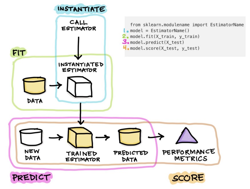
The following image will describe the whole process better as to how the learning algorithm function in scikit-learn works.
Source: https://miro.medium.com/max/875/1*NGPAHYYqs6yRUhMj2BbLaw.jpeg
The overall processes can be divided into the following steps which can be summarized as follows :
Step 1: We first need to import an estimator function from the module of scikit-learn. An estimator is actually a learning algorithm like RandomForestClassifier which can then be used to train the data and then predict the values
Step 2: We need to then instantiate the estimator model and this can be done by assigning it to a variable. The name can be any but as a standard convenience, we use some specific names for the models.
Step 3: Now we move onto model training or model building which will allow the model to learn from the training dataset values. The training is done with the fit() function where the data is supplied as the argument of the mode. Generally, the data which has already been divided into training and test data, only the training data is used to train the model.
Step 4: After training the model, it will be used to make predictions based on a totally new and unseen dataset. This is all done with the help of predict() function. The predicted values are stored in a separate variable which can be used to compute the efficiency of a model.
Step 5: The most simple and easy way to calculate the score of a function is to use the .score() function. In a regression model, the score function is used to calculate the R2 value.
For more functionality, we can add some more steps to it and that would extend the core workflow and include other steps which would boost the robustness and improve the ways in which the model can be used.
2. How to Interpret the model
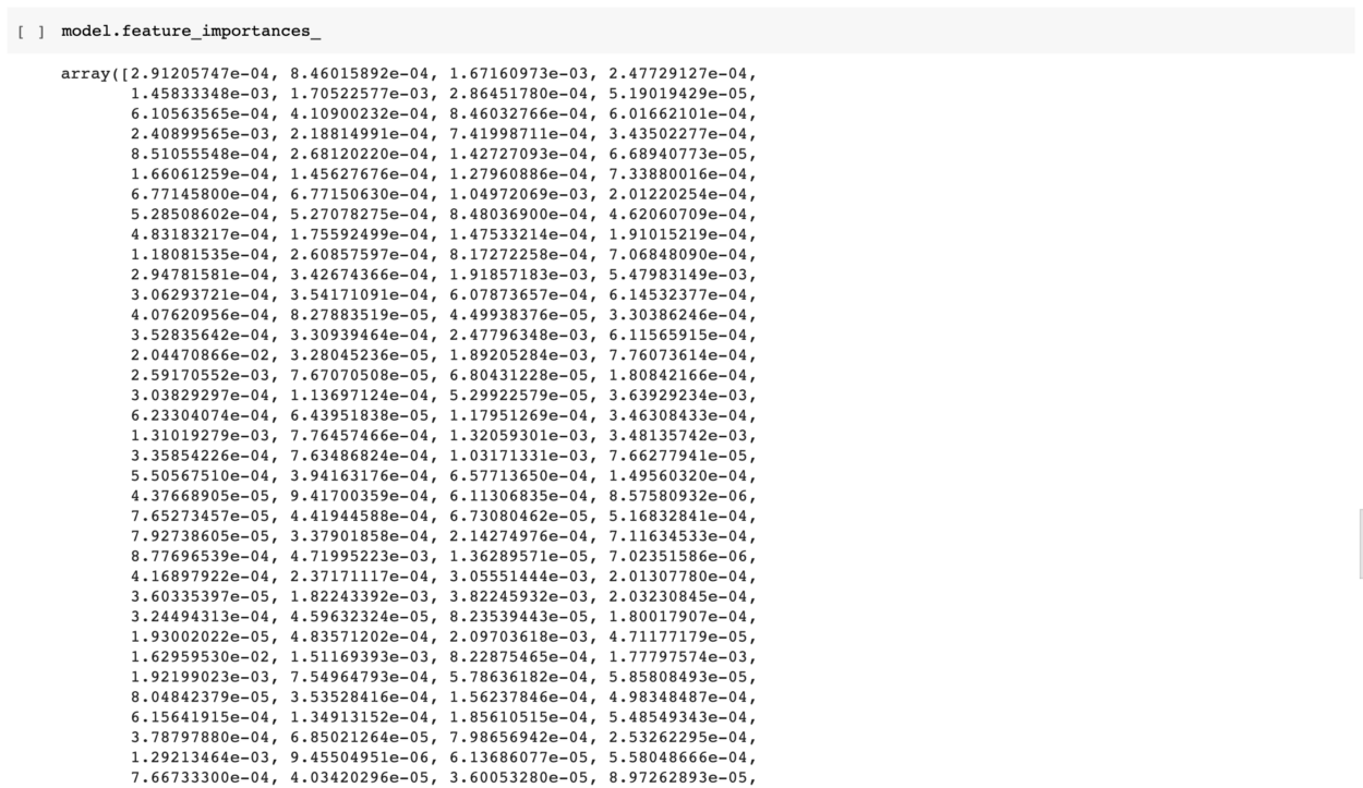
Not all models are useful and only when valuable insights can be interpreted from the data and model, it is considered to be a good model. The features which are important for a model are stored in a model and can always be extracted. We can do that by the following attribute of the model
Code :
rf.feature_importances_
Output :
array([0.03181313, 0.0301273 , 0.06371387, 0.02197285, 0.02890615,
       0.02184419, 0.62510158, 0.02628674, 0.11794592, 0.03228826])
It will give us an array of important values of the various features which are used in the model. Putting this back in our initial code :
We can mix this with the dataframe names and then give a cleaner output.
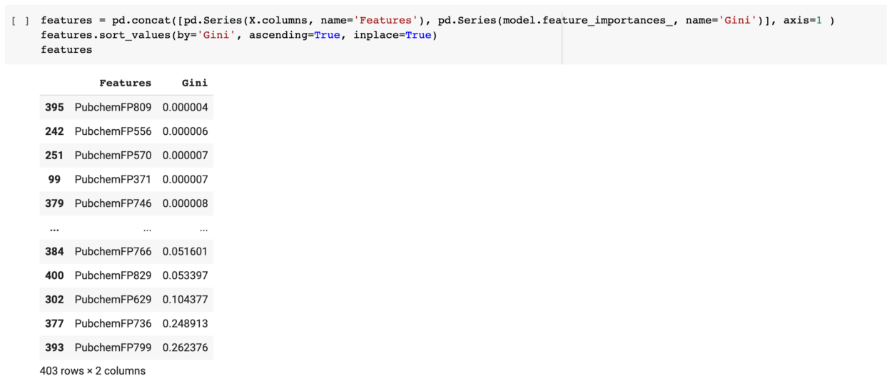
We can also create a feature important plot from the model as given below.
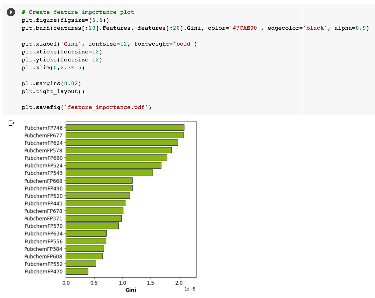
So in a nutshell, we can see that the name implies that the feature important plot shows a more detailed result as to how each feature is important as judged from the obtained Gini indexes from the random forest model.
3. How to do Hyperparameter Tuning
For the first few models of anyone, you can use the default hyperparameters. Initially, the first few attempts will be to make sure that the models get trained and predict perfectly but after that when you are comfortable with your skills. It’s time t move to the next step which is to make the model even better by tuning the hyperparameters.
Let’s stick to a basic machine learning model like a random forest and it will also provide a balance between model interpretability and robust performance. First, you need to make sure your model is in place and working and then you can work on its hyperparameter tuning to maximize the results of the model.
A random forest algorithm works very well on its own but it does not achieve very high accuracy on its own and hence tuning is necessary for it. For other algorithms like Support Vector Machine, it is crucial for hyperparameter tuning to reach a robust performance. We will tune out the model with the help of the ” GridSearchCV() ” function.
1. We will first create an artificial Dataset, split the data and then train and test to build the base and improve it as we proceed.
Code :
from sklearn.datasets import make_classification
X, Y = make_classification(n_samples=200, n_classes=2, n_features=10, n_redundant=0, random_state=1)
from sklearn.model_selection import train_test_split
X_train, X_test, y_train, y_test = train_test_split(X, Y, test_size=0.2)
from sklearn.ensemble import RandomForestClassifier
rf = RandomForestClassifier(max_features=5, n_estimators=100)
rf.fit(X_train, y_train)
rf.predict(X_test)
rf.score(X_test, y_test)
Output :
0.825
2. We will do hyperparameter tuning using GridSearchCV() in the following manner :
Code :
from sklearn.model_selection import GridSearchCV
import numpy as np
max_features_range = np.arange(1,6,1)
n_estimators_range = np.arange(10,210,10)
param_grid = dict(max_features=max_features_range, n_estimators=n_estimators_range)
rf = RandomForestClassifier()
grid = GridSearchCV(estimator=rf, param_grid=param_grid, cv=5)
grid.fit(X_train, Y_train)
Output :
GridSearchCV(cv=5, error_score=nan,
             estimator=RandomForestClassifier(bootstrap=True, ccp_alpha=0.0,
                                              class_weight=None,
                                              criterion='gini', max_depth=None,
                                              max_features='auto',
                                              max_leaf_nodes=None,
                                              max_samples=None,
                                              min_impurity_decrease=0.0,
                                              min_impurity_split=None,
                                              min_samples_leaf=1,
                                              min_samples_split=2,
                                              min_weight_fraction_leaf=0.0,
                                              n_estimators=100, n_jobs=None,
                                              oob_score=False,
                                              random_state=None, verbose=0,
                                              warm_start=False),
             iid='deprecated', n_jobs=None,
             param_grid={'max_features': array([1, 2, 3, 4, 5]),
                         'n_estimators': array([ 10,  20,  30,  40,  50,  60,  70,  80,  90, 100, 110, 120, 130,
       140, 150, 160, 170, 180, 190, 200])},
             pre_dispatch='2*n_jobs', refit=True, return_train_score=False,
             scoring=None, verbose=0)
Code :
print("The best parameters are %s with a score of %0.2f"
      % (grid.best_params_, grid.best_score_))
Output :
The best parameters are {'max_features': 1, 'n_estimators': 90} with a score of 0.91
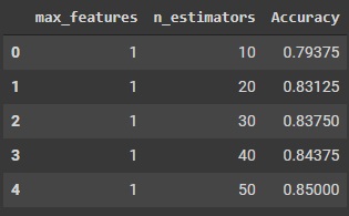
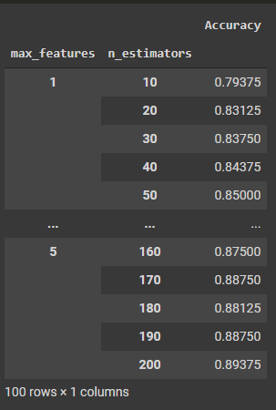
Code :
import pandas as pd
grid_results = pd.concat([pd.DataFrame(grid.cv_results_["params"]),pd.DataFrame(grid.cv_results_["mean_test_score"], columns=["Accuracy"])],axis=1)
grid_results.head()
Output :
Code :
grid_contour = grid_results.groupby(['max_features','n_estimators']).mean()
grid_contour
Output :
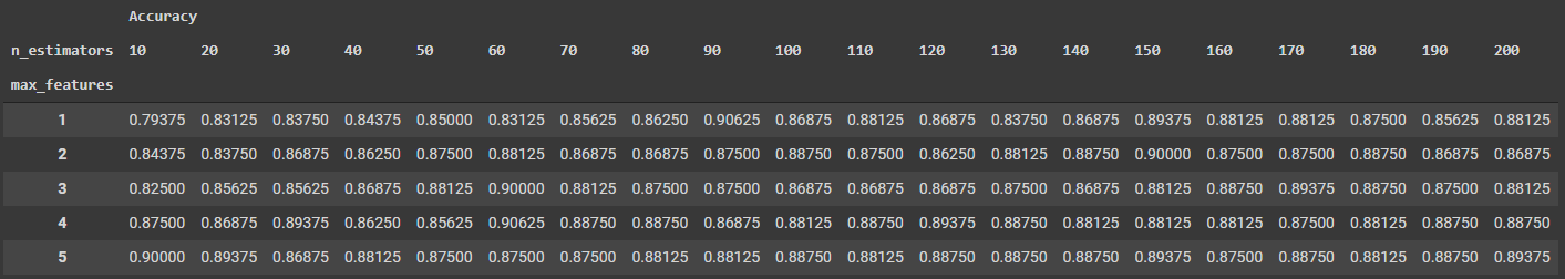
Code :
grid_reset = grid_contour.reset_index()
grid_reset.columns = ['max_features', 'n_estimators', 'Accuracy']
grid_pivot = grid_reset.pivot('max_features', 'n_estimators')
grid_pivot
Output :
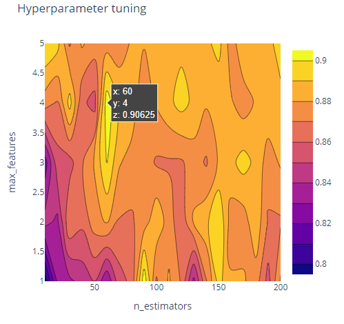
3. Now we will display the results got from hyperparameter tuning in a visual manner
Code :
x = grid_pivot.columns.levels[1].values
y = grid_pivot.index.values
z = grid_pivot.values
import plotly.graph_objects as go
layout = go.Layout(
            xaxis=go.layout.XAxis(
              title=go.layout.xaxis.Title(
              text='n_estimators')
             ),
             yaxis=go.layout.YAxis(
              title=go.layout.yaxis.Title(
              text='max_features')
            ) )
fig = go.Figure(data = [go.Contour(z=z, x=x, y=y)], layout=layout )
fig.update_layout(title='Hyperparameter tuning', autosize=False,
                  width=500, height=500,
                  margin=dict(l=65, r=50, b=65, t=90))
fig.show()
Output :
Code :
import plotly.graph_objects as go
fig = go.Figure(data= [go.Surface(z=z, y=y, x=x)], layout=layout )
fig.update_layout(title='Hyperparameter tuning',
                  scene = dict(
                    xaxis_title='n_estimators',
                    yaxis_title='max_features',
                    zaxis_title='Accuracy'),
                  autosize=False,
                  width=800, height=800,
                  margin=dict(l=65, r=50, b=65, t=90))
fig.show()
Output :
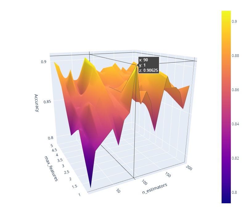
Here we can see a 3D plot of the tuning results with respect to the no of estimators and the max features. For our model, the maximum efficiency is 0.90625 and it can be achieved through 2 different points according to the results we have got. Can you find them both? Share the article with 2 of your friends and reach out to me on LinkedIn or Gmail stating the 2 different points for which we get a 0.90625 score if you are paying attention, and we can talk more scikit-learn or maybe give a small monetary reward for the find.
Bonus Material: Resources for Scikit-Learn
Everyone finds it helpful if they can find all the necessary information on one page and remembering them all can be quite challenging. So some cheatsheets can help you to remember and use scikit tools better which are :
Documentation: You can find the API documentation, examples, and the user guide which are provided on their website for free.
Cheat Sheet: From their official website you can get a handy cheat sheet where you can effectively choose the correct algorithm for your task and you will be taken to a page of that algorithm when you click on it.
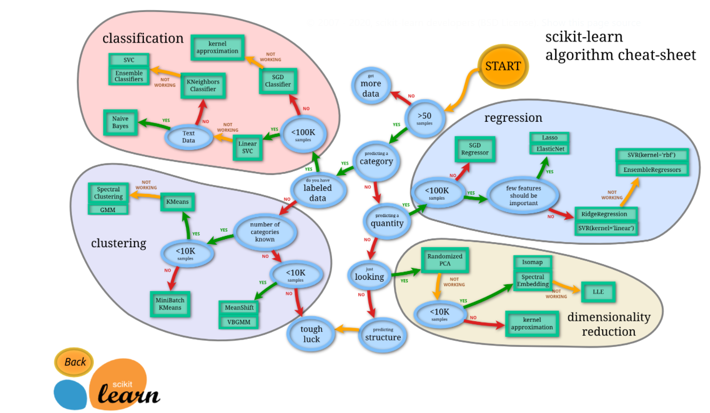
Source: https://scikit-learn.org/stable/tutorial/machine_learning_map/index.html
Books: You can find many good books on Amazon and also online for free which will help you learn about scikit-learn. You can make it your occasional habit of reading it in your leisure time. My personal favourite is the book ” The Python Data Science Handbook” which is by Jake VanderPlas which starts from NumPy, pandas and goes up to scikit-learn. A free online version of the book is available here and all the notebooks mentioned in the book are available here.
End Notes
So that is is for this article and we will discuss more on how to work on the data and transform and process it in Part -2 of the article and so stay tuned and updated. I will be publishing it soon. Stay safe everyone
Author – Ankita Roy
Blog – https://www.analyticsvidhya.com/blog/author/b_95_ankita2140664/
https://colab.research.google.com/drive/1Uovt0qXscUcYfoghZqO6av8fpveUfSb1?usp=sharing


