Holt Winter’s Method for Time Series Analysis

This article was published as a part of the Data Science Blogathon

Introduction to Time Series Analysis

Time Series Analysis is the most widely used field of data science and machine learning, it decomposes the past historical data to depict the trend, seasonality, and noise to derive the future trends from it. It’s a type of predictive analysis that forecasts the value of a variable in future occurrences based on history. The predicted values can be influenced by certain external factors which are known as independent variables like in the case of sale of a product is influenced by the discount percentage on its prices or the temperature on a particular day is influenced by the humidity or wind speed etc.

There are a number of time series forecasting algorithms available to a data scientist but the choice of algorithm depends on the business problems and the data set at hand. From simple time series forecasting techniques like moving average, exponential smoothing, ARIMA, etc to deep learning forecasting methods like recurrent neural networks, long short term memory, XG Boost, gradient boosting, fuzzy time series algorithms, etc can be used for analysis.

Along with this algorithm, hybrid forecasting techniques are also used which combine the new approaches and have been improved to obtain more accurate forecast results. A combination of two or more techniques for forecasting is known as hybrid forecasting techniques.

Image Source: Google Images https://www.bounteous.com/insights/2020/09/15/forecasting-time-series-model-using-python-part-two/

What is holt winter’s method?

Real-world data like that of demand data in any industry generally has a lot of seasonality and trends. When forecasting demands in such cases requires models which will account for the trend and seasonality in the data as the decision made by the business is going to be based on the result of this model. For such cases, Holt winter’s method is one of the many time series prediction methods which can be used for forecasting.

Holt-Winter’s Exponential Smoothing as named after its two contributors: Charles Holt and Peter Winter’s is one of the oldest time series analysis techniques which takes into account the trend and seasonality while doing the forecasting. This method has 3 major aspects for performing the predictions. It has an average value with the trend and seasonality. The three aspects are 3 types of exponential smoothing and hence the hold winter’s method is also known as triple exponential smoothing.

Let us look at each of the aspects in detail.

Exponential Smoothing: Simple exponential smoothing as the name suggest is used for forecasting when the data set has no trends or seasonality.

Holt’s Smoothing method: Holt’s smoothing technique, also known as linear exponential smoothing, is a widely known smoothing model for forecasting data that has a trend.

Winter’s Smoothing method: Winter’s smoothing technique allows us to include seasonality while making the prediction along with the trend.

Hence the Holt winter’s method takes into account average along with trend and seasonality while making the time series prediction.

Forecast equation^yt+h|t=ℓt+hbt

Level equationℓt=αyt+(1−α)(ℓt−1+bt−1)

Trend equationbt=β∗(ℓt−ℓt−1)+(1−β∗)bt−1

Where ℓtℓt is an estimate of the level of the series at time tt,

btbt is an estimate of the trend of the series at time tt,

αα is the smoothing coefficient

Example with code

Let us look at Holt-Winter’s time series analysis with an example. We have the number of visitors on a certain website for few days, let us try to predict the number of visitors for the next 3 days using the Holt-Winter’s method. Below is the code in python

The first step to any model building is exploratory data analysis or EDA, lets look at the data and try to clean it before fitting a model onto it.

Missing values Treatment

#counting the number of missing data points
visitors = pd.read_excel('website_visitors.xlsx',index_col='month', parse_dates=True)
Visitors_df_missing = (visitors.[ 'no_of_visits']=nan).sum()
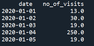
Print(Visitors.head())

#Replace the missing values with the mean value
visitors ['no_of_visits'].fillna(value= visitors ['no_of_visits'].mean(), inplace=True)

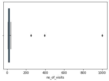
Outlier detection and treatment

import seaborn as sns
 sns.boxplot(x= visitors ['no_of_visits'])

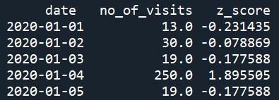
#calculating the z score

visitors [‘z_score’] = visitors. 'no_of_visits' - visitors. 'no_of_visits'.mean())/visitors. 'no_of_visits'.std(ddof=0)

#exclude the rowl with z score more than 3
visitors [(np.abs(stats.zscore(visitors [‘z_score’])) < 3)]

#re-sampling the data to monthly buckets
visitors.set_index('date', inplace=True)
visitors.resample('MS').sum()

Now our EDA is completed and the data set is ready for modelling

# Lets import all the required libraries

import pandas as pd
from matplotlib import pyplot as plt
from statsmodels.tsa.seasonal import seasonal_decompose
from statsmodels.tsa.seasonal import seasonal_decompose 
from statsmodels.tsa.holtwinters import SimpleExpSmoothing   
from statsmodels.tsa.holtwinters import ExponentialSmoothing

# Input the visitors data using pandas
visitors = pd.read_excel('website_visitors.xlsx',index_col='month', parse_dates=True)
print(visitors.shape)
print(visitors.head()) # print the data frame
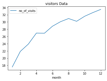
visitors[['no_of_visits']].plot(title='visitors Data')

visitors.sort_index(inplace=True) # sort the data as per the index

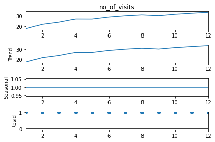
# Decompose the data frame to get the trend, seasonality and noise
decompose_result = seasonal_decompose(visitors['no_of_visits'],model='multiplicative',period=1)
decompose_result.plot()
plt.show()

# Set the value of Alpha and define x as the time period
x = 12
alpha = 1/(2*x)

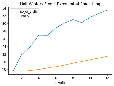
# Single exponential smoothing of the visitors data set
visitors['HWES1'] = SimpleExpSmoothing(visitors['no_of_visits']).fit(smoothing_level=alpha,optimized=False,use_brute=True).fittedvalues      
visitors[['no_of_visits','HWES1']].plot(title='Holt Winters Single Exponential Smoothing grpah')

# Double exponential smoothing of visitors data set ( Additive and multiplicative)

visitors['HWES2_ADD'] = ExponentialSmoothing(visitors['no_of_visits'],trend='add').fit().fittedvalues
visitors['HWES2_MUL'] = ExponentialSmoothing(visitors['no_of_visits'],trend='mul').fit().fittedvalues
visitors[['no_of_visits','HWES2_ADD','HWES2_MUL']].plot(title='Holt Winters grapg: Additive Trend and Multiplicative Trend')

# Split into train and test set
train_visitors = visitors[:9]
test_visitors = visitors[9:]

# Fit the model
fitted_model = ExponentialSmoothing(train_visitors['no_of_visits'],trend='mul',seasonal='mul',seasonal_periods=2).fit()
test_predictions = fitted_model.forecast(5)
train_visitors['no_of_visits'].plot(legend=True,label='TRAIN')
test_visitors['no_of_visits'].plot(legend=True,label='TEST',figsize=(6,4))
test_predictions.plot(legend=True,label='PREDICTION')
plt.title('Train, Test and Predicted data points using Holt Winters Exponential Smoothing')

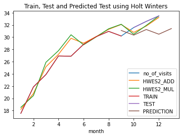
Basically, there are 2 models multiplicative and additive. The additive model is based on the principle that the forecasted value for each data point is the sum of the baseline values, its trend, and the seasonality components.

Similarly, the multiplicative model calculates the forecasted value for each data point as the product of the baseline values, its trend, and the seasonality components.

Limitations of Holt-Winter’s Technique

In spite of giving the best forecasting result the Holt-Winter’s method still has certain shortcomings. One major limitation of this algorithm is the multiplicative feature of the seasonality. The issue of multiplicative seasonality is how the model performs when we have time frames with very low amounts. A time frame with a data point of 10 or 1 might have an actual difference of 9 but there is a relative difference of about 1000%, so the seasonality, which is expressed as a relative term could change drastically and should be taken care of of of when building the model.

FOOTNOTES:

Holt winter’s algorithm has wide areas of application. It is used in various business problems mainly because of two reasons one of which is its simple implementation approach and the other one is that the model will evolve as our business requirements change.

Holt Winter’s time series model is a very powerful prediction algorithm despite being one of the simplest models. It can handle the seasonality in the data set by just calculating the central value and then adding or multiplying it to the slope and seasonality, We just have to make sure to tune in the right set of parameters, and viola, we have the best fitting model. Always remember to check the efficiency of the model using the MAPE (mean absolute percentage error) value or the RMSE(Root mean squared error) value, and the accuracy may depend on the business problem and the data set available to train and test the model.