This article was published as a part of the Data Science Blogathon
What is Linear Regression?
Regression is a statistical term for describing models that estimate the relationships among variables.
Linear Regression model study the relationship between a single dependent variable Y and one or more independent variable X.
If there is only one independent variable, it is called simple linear regression, if there is more than one independent variable then it is called multiple linear regression.
It is modelling between the dependent and one independent variable. When there is only one independent variable in the linear regression model, the model has generally termed a simple linear
regression model.
The basic algorithm to predict values for all machine learning models is the same.
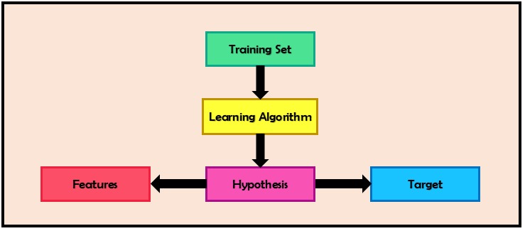
Hypothesis
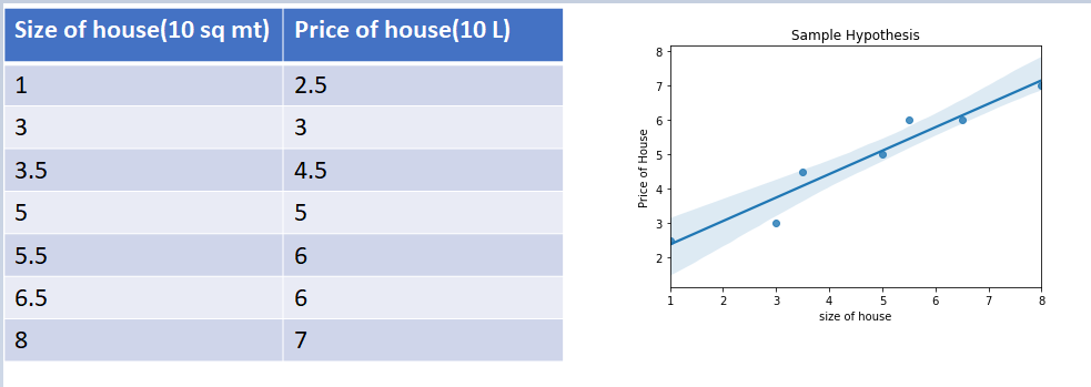
Now let’s consider a model with one independent feature(x) and a sample training set where the dependent feature is the size of the house(x) and the prediction is the price of the house(y).
As we know that in this case (y) is linearly dependent on (x) hence we can create a hypothesis that can be resembled the equation of a straight line (y=mx+c).
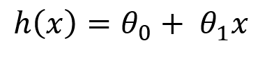
To analyze the behaviour of the formed hypothesis, assume the value of (θ₀)=2 and (θ₁)=5/8.
Here (θ₀)and (θ₁) are also called regression coefficients.
Below is the graph showing the sample dataset and hypothesis.
Now we have a major question in our mind: how to correctly choose the value of (θ₀) and (θ₁) so that our model will be accurate or predict values more precisely. So for this, we need to look at the terms which can be minimized to get the most accurate results.
The first thing which we can do is to reduce the error /difference between our hypothetical model’s predictions and the real values,
so we want to minimize the function for each valid (i), where (i) denotes a valid data entry in our data.
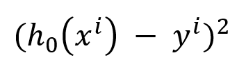
If we want to minimize the error for every value, then we need to minimize
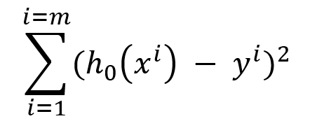
where (m) is the number of records present in our dataset
form this we can say that we need to reduce the squared error of the hypothetical model.
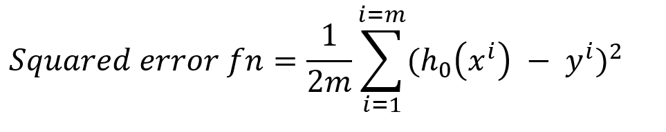
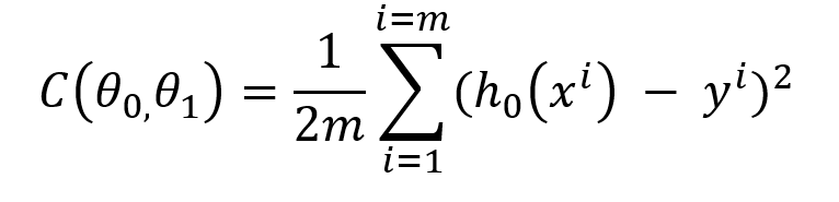
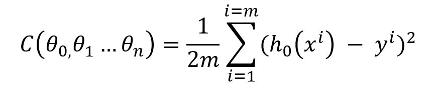
So let the squared error function be called as cost function (C) which has 2 dependent variables (θ₀) and (θ₁) and our goal is to minimize this cost function(C), for this, we will use batch gradient descent.
Gradient Descent
The technique helps to find optimal (θ₀) and (θ₁). Here is how it helps in finding the minimum cost function (optimal values of (θ₀) and (θ₁)).
- Pick random values of (θ₀) and (θ₁).
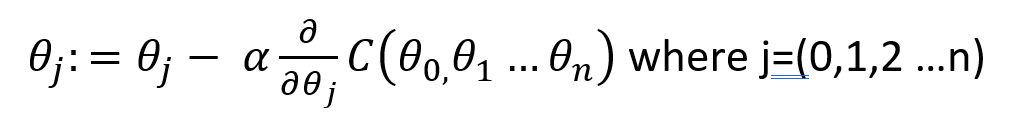
- Keep on simultaneously updating values of (θ₀) and (θ₁) till the convergence.
- If the cost function does not decrease anymore, we reached our local minima.
One important thing to note is that the value of (θ₀) and (θ₁)must be increased simultaneously which means that we can separate the values of (θ₀) and (θ₁) and update them later
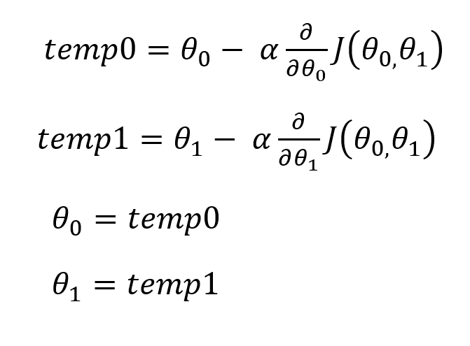
If the values don’t get updated simultaneously then, for ex: the equation of (θ₁) will get the updated value of (θ₀) and thus will provide incorrect results.
Plotting
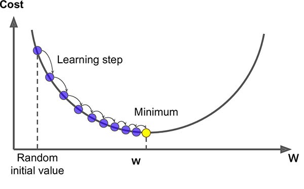
Let us first visualize using only 1 feature say (θ₁).
We will plot a graph comparing changes in C(θ₁) with changes in (θ₁).
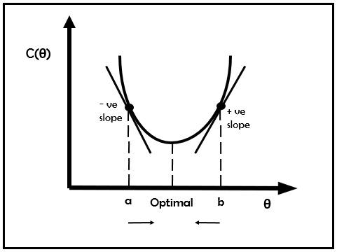
As we can see here the rate of change of (θ₀) and (θ₁) depends on what is the learning rate (α).
Now, the question is how do we choose a proper value of learning rate (α) for our model?
- If the value of (α) is too low then our model will consume time and will have slow convergence.
- If the value of (α) is too high then our (θ₀) and (θ₁) may overshoot the optimal value and hence accuracy of the model will decrease.
- It is also possible in the high value of (α) that (θ₀) and (θ₁) will keep on bouncing between 2 values and may never reach the optimal value.
Generally, the value of (α) then depends on a range of our dependent variables.
We can’t have the same value of (α) for x ranging from 1 to 10,00,000 and 0.01 to 0.001.
So it makes sense to choose the value of (α) relative to (x). In most of the cases, (α) = x * 10 ^(-3).
Also, one thing to notice here is, even by putting the constant value of (α), the change in the value of (θ₀) and (θ₁) will decrease in every step because the slope of gradient descent will be decreasing as values of (θ₀) and (θ₁) approaches to minimum values.
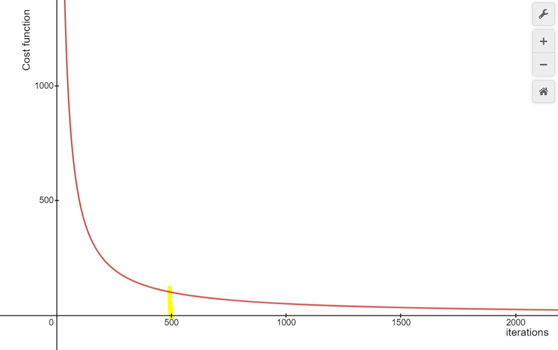
The plot of the Cost function (C) vs several iterations taken to reach minima must be like the graph shown below. Here around 500 iterations will be taken by the model to reach the approximate minima and after that, the graph will eventually flatten out.
If any other graph is plotted not similar to this, then (α) must be reduced.
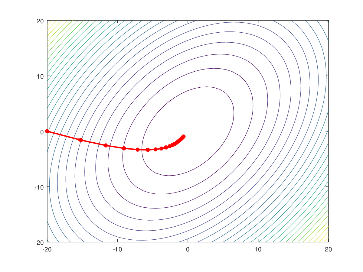
Generally in plotting a graph of 3 axes (C(cost function), (θ₀),(θ₁)), we will get a bowl-shaped graph, hence there will be only 1 minimum in the entire plot.
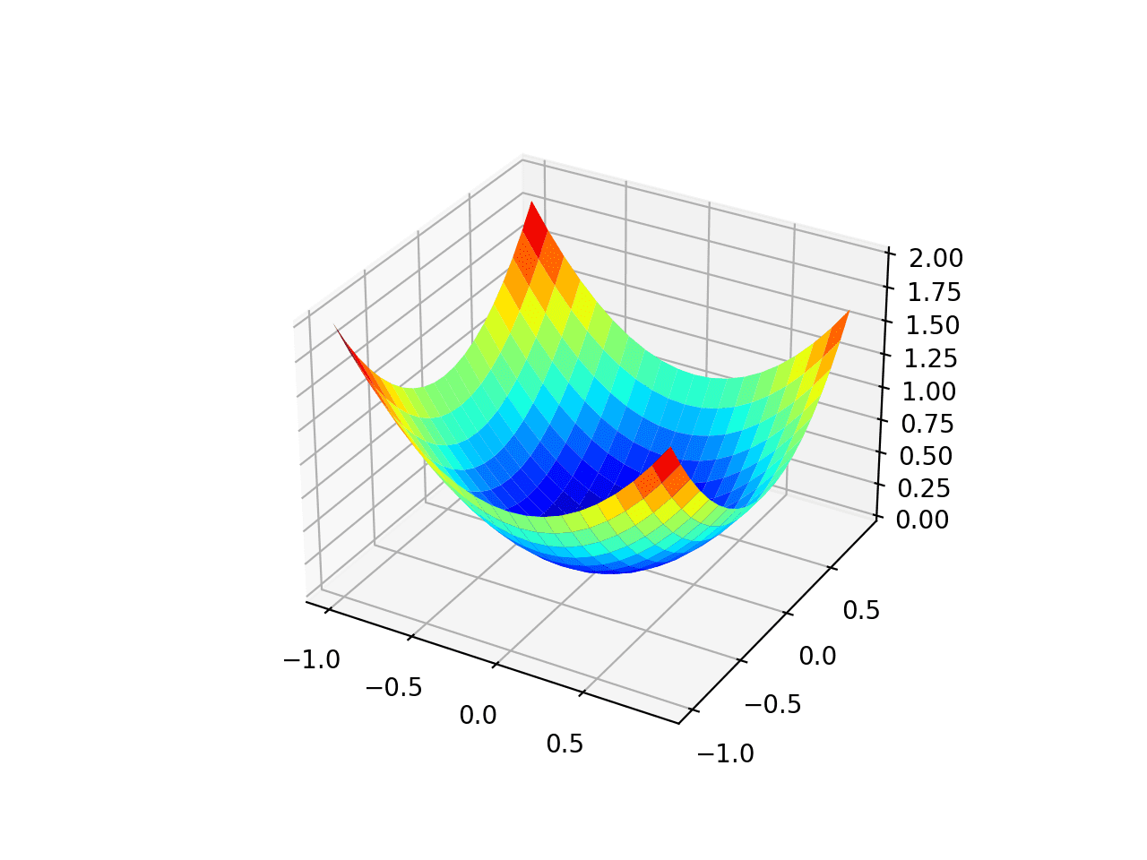
For ease of visualization, we plot the contour graph of the following data, the contour will have a unique centre because of the single minima present in the graph and the centre of the contour plot will give us an optimal value of (θ₀) and (θ₁).
So now we have all the necessary equations and values to make a hypothesis that best fits the Linear Regression problem.
To improve the model, we can make 2 modifications.
- Learn with a larger number of features (Implement Multilinear Regression).
- Solve for (θ₀) and (θ₁) without using an iterative algorithm like gradient descent.
Multi Linear Regression
In MLR, we will have multiple independent features (x) and a single dependent feature (y). Now instead of considering a vector of (m) data entries, we need to consider the (n X m) matrix of X, where n is the total number of dependent features.
So let us extend these observations to gain insights on Linear regression with multiple features or Multi-Linear Regression.
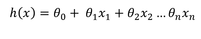
Firstly our hypothesis will change to n features now instead of just 1 feature.
But firstly in the case of Multiple Linear Regression, the most important thing is to make sure that all the features are on the same scale.
We do not want a model where one feature varies from 1 to 10000 and the other in a range of 0.1 to 0.01.
hence it is important to scale the features before making any hypothesis.
Feature Scaling
There are many ways to achieve feature scaling, the method which I am going to discuss here is Mean Normalisation.
As the name itself suggest, the mean of all features is approximately 0.
The formula to calculate normalized values is
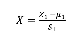
Where (u) is the average value of (X₁) in the training set,(S₁) is the range of values.
(S₁) can also be chosen as Standard Deviation of (X₁), the values will still be normalized but the range will change.
In MLR now our cost function will be modified to
And the Gradient descent simultaneous update will change to
Normal Equation
We know that batch gradient descent is an iterative algorithm, it uses all the training set at each iteration.
But gradient descent works better for larger values of n and is preferred over normal equations in large datasets.
Instead, Normal Equation makes use of vectors and matrices to find us minimum values.
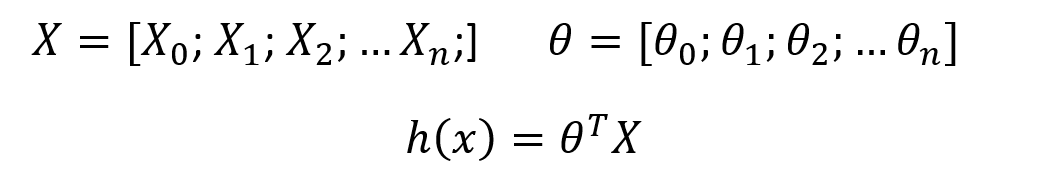
in our hypothesis, we have values of (θ) as well as (x) ranging from 0 to n, so we create vectors individually of (θ) and (x) and our hypothesis formed will be,
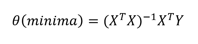
To find minimum values of (θ) to reduce the cost function, and skipping the steps of gradient descent like to choose a proper learning rate (α), to visualize plots like contour plots or 3D plots and without feature scaling, the optimal values of (θ) can be calculated as
Key features of Normal Equation
- No need to choose learning rate (α)
- No iterations
- Feature scaling is not important
- Slow if there are a large number of features(n is large).
- Need to compute matrix multiplication (O(n3)). cubic time complexity.
gradient descent works better for larger values of n and is preferred over normal equations in large datasets.
We can also extend the concept of multilinear regression to form our base for the polynomial Regression.
Conclusion
In conclusion, for our model to perform accurately using gradient descent, values of (θ₀),(θ₁), and (α) play a major role. There can be many techniques as a normal equation which is comparatively easier to implement is used to find correct values of (θ₀) and (θ₁) but the most accurate result in a larger number of features is achieved by using Gradient descent.
Hope this article provided some new insights and an idea of how a simple looking model like linear regression is supported by pure mathematical concepts!
Keep Learning, Keep exploring!


