This article was published as a part of the Data Science Blogathon
Dear readers,
In this blog, we will build a random forest classifier(RFClassifier) model to detect breast cancer using this dataset from Kaggle. We will then apply some of the popular hyperparameter tuning techniques to this basic model in order to arrive at the optimal model which exhibits the best performance by thoroughly comparing the results of all the hyperparameter optimization techniques applied. I have covered both basic and advanced techniques of hyperparameter optimization in this blog. Not only the step-by-step implementation but, I have also discussed the underlying theory of each of the following hyperparameter tuning techniques which we will look at, in a while:
Basic Techniques:
- RandomizedSearchCV
- GridSearchCV
Advanced Techniques:
- Bayesian Optimization
- TPOT Classifier(Genetic Algorithm)
- Optuna
So, let us begin…
Agenda
- What do you mean by the term hyperparameter optimization and why is it essential?
- Pre-processing of the dataset
- Train-test split
- Building a basic RFClassifier model
- Manual hyperparameter tuning
- What is RandomizedSearchCV?
- Hyperparameter tuning using RandomizedSearchCV
- What is GridSearchCV?
- Hyperparameter tuning using GridSearchCV
- How to choose between GridSearchCV and RandomizedSearchCV
- What is Bayesian Optimization?
- Hyperparameter tuning using Bayesian Optimization
- What is TPOT Classifier?
- Hyperparameter tuning using TPOT Classifier
- What is the Genetic Algorithm?
- What is Optuna?
- Hyperparameter tuning using Optuna
- Results of the models
What do you mean by the term hyperparameter optimization and why is it essential?
The goal of hyperparameter optimization is to optimize the target value and thus obtain the best solution among all the possible solutions out there. Several packages such as GridSearchCV, RandomizedSearchCV,optuna and so on greatly help us tune our models by identifying the best combination from the combinations of hyperparameters given by us. These packages are thus termed hyperparameter tuning or, alternatively, hyperparameter optimization techniques. Don’t worry, we will be looking at each of them very much in detail in the upcoming sections of the blog.
If we do not assign any values for the parameters, quite obviously, as one might easily guess, the default values will be considered. But, the question here is, to what extent will these default values be applicable for the given dataset? This is indeed something serious to think about while building a model. Also, the values of these parameters cannot be simply guessed randomly as if we were playing a game just for time-pass!
Summing up, these parameters must be given values based on a technique, popularly referred to as “Hyperparameter Optimization”.
Above all, hyperparameter optimization is highly essential while working with larger datasets. However, in the case of a small dataset, it causes only slight changes in the model’s accuracy. A practical use-case of hyperparameter optimization includes the continuous monitoring of an ML model after it is deployed and users start using it extensively. Based on its live performance, the developers must decide if their model needs further hyperparameter tuning.
Pre-processing of the dataset
Before we kickstart the most awaited section of the blog-the implementation, I would like to repeat that I have used this dataset throughout the implementation. So, quite obviously, you need to head on to the link and download the dataset! Also, I have used Google Colab for the entire implementation.
Let’s begin, as always, by importing the necessary packages:
import warnings
warnings.filterwarnings('ignore')
The above code improves the presentation of our outputs by ignoring warnings. Lets now read the CSV file using pandas and understand our dataset:
import numpy as np
import pandas as pd
df=pd.read_csv('data.csv')
df.info()
On executing the above code, it is observed that our dataset consists of 569 rows and 33 columns, in all. Now, check for the presence of any missing values:
df.isna().sum()
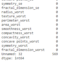
Oh my goodness! Just look at the last column named “Unnamed: 32”!It only consists of NaN(missing values). Hence, as it is completely useless, we can simply drop it without any hesitation:
df=df.drop('Unnamed: 32',axis=1)
Next, let us proceed to understand the diagnosis column:
df['diagnosis'].value_counts()
#B-benign and M-malignant
Running the above code, it is observed that the dataset consists of 357 cases of benign(B) and the rest 212 being malignant(M).
Now, we have to do the feature selection. Note that the column namely ‘id’ is not useful. Just because a patient has id 100, it cannot be concluded that she suffers from breast cancer! So, let’s simply drop it using the below code:
df=df.drop('id',axis=1)
Observe that, in this example, we are planning to build an RFClassifier to predict if a given case comes under the category of B or M.Thus, the diagnosis column becomes our target variable(Y) and all the other columns are our inputs(features) denoted by the variable X.
X=df.drop('diagnosis',axis=1)
y=df['diagnosis']
Train-test split
Now, let’s set out to divide our dataset into 2 parts-train and test. As you might have already known, the training dataset is used to train our model. The trained model is then tested with the completely unseen dataset which is nothing but the test dataset. You can choose the split ratio at your convenience. Anyways, I have chosen the most advisable split ratio as follows:80% for train and the rest 20% for test.
#### Train Test Split
from sklearn.model_selection import train_test_split
X_train,X_test,y_train,y_test=train_test_split(X,y,test_size=0.20,random_state=0)
Building a basic RFClassifier model
Creating an RFClassifier model is easy. All you have to do is to create an instance of the RandomForestClassifier class as shown below:
from sklearn.ensemble import RandomForestClassifier
rf_classifier=RandomForestClassifier().fit(X_train,y_train)
prediction=rf_classifier.predict(X_test)
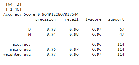
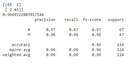
Now, it’s time to analyze its performance using confusion matrix,accuracy_score, and classification report.
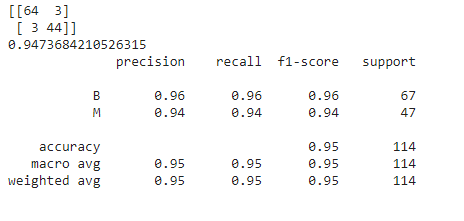
from sklearn.metrics import confusion_matrix,classification_report,accuracy_score
print(confusion_matrix(y_test,prediction))
print(accuracy_score(y_test,prediction))
print(classification_report(y_test,prediction))
The output for the above code is as follows:
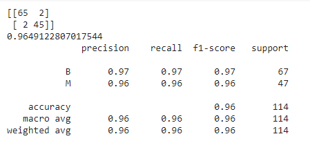
Note that, for the above model, we have not set any parameters which means that by default, the default values of these parameters have been taken into consideration. Thus, the above is the performance of our model with respect to the default parameters. How good is it? What do you think about it?
Manual Hyperparameter Optimization
Before directly jumping into the techniques, let us first have a look at the main parameters of RFClassifier which we will be tuning in this blog:
- criterion
- max_depth
- max_features
- max_samples_leaf
- min_samples_split
- n_estimators
criterion:
It is a function that tells how good the split is. Split, in this context, does not refer to the train-test split which we did earlier! Instead, it refers to the splitting of a node of a decision tree.
Note that RFClassifier has a number of decision trees and it uses ensembling techniques to predict
max_depth:
It refers to the number of levels that each tree can have, at the most.
max_features:
It refers to the number of features that can be considered, at the most, while splitting a node.
min_samples_leaf:
It refers to the number of samples that a leaf can store, at the least.
min_samples_split:
It refers to the minimum number of samples required within a node to lead to the splitting of the node.
n_estimators:
It refers to the number of trees that the ensemble has.
I hope that by now you have some brief idea about the parameters which we will be tuning in all the techniques. Hence, we are all good to start off with the manual hyperparameter tuning! For this, we will just set some random values to these parameters while creating the model and thus look at our new model’s performance. Here, by new model, I meant the model created by passing these values to the parameters as shown below:
### Manual Hyperparameter Tuning
model=RandomForestClassifier(n_estimators=300,criterion='entropy',max_depth=100,min_samples_split=4,
                             max_features='sqrt',min_samples_leaf=10,random_state=100).fit(X_train,y_train)
predictions=model.predict(X_test)
print(confusion_matrix(y_test,predictions))
print(accuracy_score(y_test,predictions))
print(classification_report(y_test,predictions))
In GridSearchCV and RandomizedSearchCV,CV stands for ‘Cross validation’.This is done in order to understand,from various subsets of the data,if our model is performing well.
What is RandomizedSearchCV?
RandomizedSearchCV is the hyperparameter optimization or tuning technique in which only a few combinations are randomly selected from the given set of combinations. The algorithm is then run only for these chosen combinations. It is thus a smarter approach because it does not run on all the possible combinations of the given values of hyperparameters.
Use this technique while dealing with larger datasets or when we have a lot of parameters to be tuned.RandomizedSearchCV tends to perform better when all parameters do not equally impact the performance of the model.
Hyperparameter Optimization using RandomizedSearchCV
Here, we will pass a Python list of possible values of each of the six hyperparameters of the RFClassifier discussed earlier.
from sklearn.model_selection import RandomizedSearchCV
# Number of trees in random forest
n_estimators = [int(x) for x in np.linspace(start = 200, stop = 2000, num = 10)]
# Number of features to consider at every split
max_features = ['auto', 'sqrt','log2']
# Maximum number of levels in tree
max_depth = [int(x) for x in np.linspace(10, 1000,10)]
# Minimum number of samples required to split a node
min_samples_split = [2, 5, 10,14]
# Minimum number of samples required at each leaf node
min_samples_leaf = [1, 2, 4,6,8]
# Create the random grid
random_grid = {'n_estimators': n_estimators,
               'max_features': max_features,
               'max_depth': max_depth,
               'min_samples_split': min_samples_split,
               'min_samples_leaf': min_samples_leaf,
              'criterion':['entropy','gini']}
print(random_grid)
rf=RandomForestClassifier()
rf_randomcv=RandomizedSearchCV(estimator=rf,param_distributions=random_grid,n_iter=100,cv=3,verbose=2,
                               random_state=100,n_jobs=-1)
### fit the randomized model
rf_randomcv.fit(X_train,y_train)
After checking the model’s performance with multiple combinations, although not all, RandomizedSearchCV returns the best or the optimal values of the parameters for which the model performed the best.
rf_randomcv.best_params_
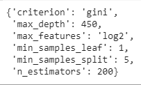
Hence, from the various values given by us for the parameters, the optimal values of the parameters, given by RandomizedSearchCV are, as shown in the above output which can be inferred in the following manner:
- criterion should be gini
- max_depth should be 450
- max_features should be log2
- min_samples_leaf must be 1
- min_samples_split should be 5
- The number of decision trees(n_estimators) should be 200.
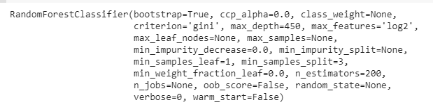
Now, we have to re-train our model passing these values given by the RandomizedSearchCV technique and then check the performance of the new model built and trained with these optimal parameters.
best_random_grid=rf_randomcv.best_estimator_
from sklearn.metrics import accuracy_score
y_pred=best_random_grid.predict(X_test)
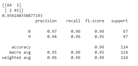
print(confusion_matrix(y_test,y_pred))
print("Accuracy Score {}".format(accuracy_score(y_test,y_pred)))
print(classification_report(y_test,y_pred))
What is GridSearchCV?
This technique fits our model on all the possible combinations of the list of parameter values given by us (unlike the previous technique) and then forms a grid. This can be easily understood with the help of the following example:
Consider that we want to tune the two parameters n_estimators and max_depth and we pass the following lists of values:
n_estimators=[10,20,30]
max_depth=[2,3]
The grid below, with the values of max_depth along rows and n_estimators along the columns, shows all the possible combinations resulting from the two lists:
|
|
|
|
|
|
|
|
|
|
|
|
Each of the cells marked ‘G’ in the above grid refers to a combination. For each of these combinations, GridSearchCV will run the RFClassifier algorithm and get accuracy. It then gives the values to be taken by the parameters to get the best model.
Hyperparameter Optimization using GridSearchCV
The procedure is the same as that of the RandomizedSearchCV technique, discussed earlier, except that, we will create our lists of values of parameters by referring to the best or optimal values of the parameters given by RandomizedSearchCV.By doing so, we reduce the number of possible combinations which GridSearchCV must take into consideration. Also, we reduce the number of iterations.
from sklearn.model_selection import GridSearchCV
param_grid = {
    'criterion': [rf_randomcv.best_params_['criterion']],
    'max_depth': [rf_randomcv.best_params_['max_depth']],
    'max_features': [rf_randomcv.best_params_['max_features']],
    'min_samples_leaf': [rf_randomcv.best_params_['min_samples_leaf'],
                         rf_randomcv.best_params_['min_samples_leaf']+2,
                         rf_randomcv.best_params_['min_samples_leaf'] + 4],
    'min_samples_split': [rf_randomcv.best_params_['min_samples_split'] - 2,
                          rf_randomcv.best_params_['min_samples_split'] - 1,
                          rf_randomcv.best_params_['min_samples_split'],
                          rf_randomcv.best_params_['min_samples_split'] +1,
                          rf_randomcv.best_params_['min_samples_split'] + 2],
    'n_estimators': [rf_randomcv.best_params_['n_estimators'] - 200, rf_randomcv.best_params_['n_estimators'] - 100,
                     rf_randomcv.best_params_['n_estimators'],
                     rf_randomcv.best_params_['n_estimators'] + 100, rf_randomcv.best_params_['n_estimators'] + 200]
}
#### Fit the grid_search to the data
rf=RandomForestClassifier()
grid_search=GridSearchCV(estimator=rf,param_grid=param_grid,cv=10,n_jobs=-1,verbose=2)
grid_search.fit(X_train,y_train)
Let’s now look at the optimal values of the parameters returned by this technique.
best_grid=grid_search.best_estimator_
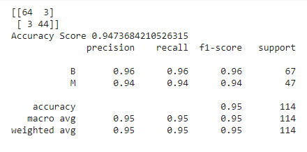
Now, we have to re-train our model with these optimal values and then check its performance:
y_pred=best_grid.predict(X_test)
print(confusion_matrix(y_test,y_pred))
print("Accuracy Score {}".format(accuracy_score(y_test,y_pred)))
print(classification_report(y_test,y_pred))
How to choose between GridSearchCV and RandomizedSearchCV?
If we have too many parameters to fine-tune, then, in that case, it is not a good idea to go with GridSearchCV; instead, you should consider RandomizedSearchCV.GridSearchCV, as it considers all the combinations, runs the algorithm for comparatively many iterations, and thus it is time-consuming. The size of the grid increases with parameters. So, it is not recommended to use GridSearchCV here.
Similarly, when you have a larger dataset, go with RandomizedSearchCV and not GridSearchCV.
If all the parameters equally impact the model’s performance, use GridSearchCV as it runs the RFClassifier algorithm for all the possible combinations, and thus we will not miss out on any. Besides, if you are working with a small dataset with a maximum of 1000 or 2000 rows which has a limited number of columns as well, even in that case, it is completely acceptable to go with GridSearchCV.
It is advisable to first apply RandomizedSearchCV and then GridSearchCV, based on the best parameters given by the former. This is done because the former narrows down the search to be done by GridSearchCV.Doing so, the number of combinations for which GridSearchCV runs the algorithm also reduces.
What is Bayesian optimization?
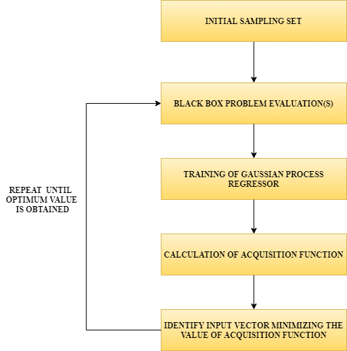
Blackbox:
It is a function inside. We are unaware of what happens inside it. We just pass input to it and it returns an output.
Training of Gaussian process regressor:
Here, we don’t train just one regression function; instead, we train a group of tuned regression functions.
Acquisition function:
It is the mathematical function describing the gain or potential optimization volume by a function. This function computes the product of standard deviation and kappa wherein kappa refers to the hyperparameter.‘ kappa‘ states if the local minimum or the global minimum was obtained.
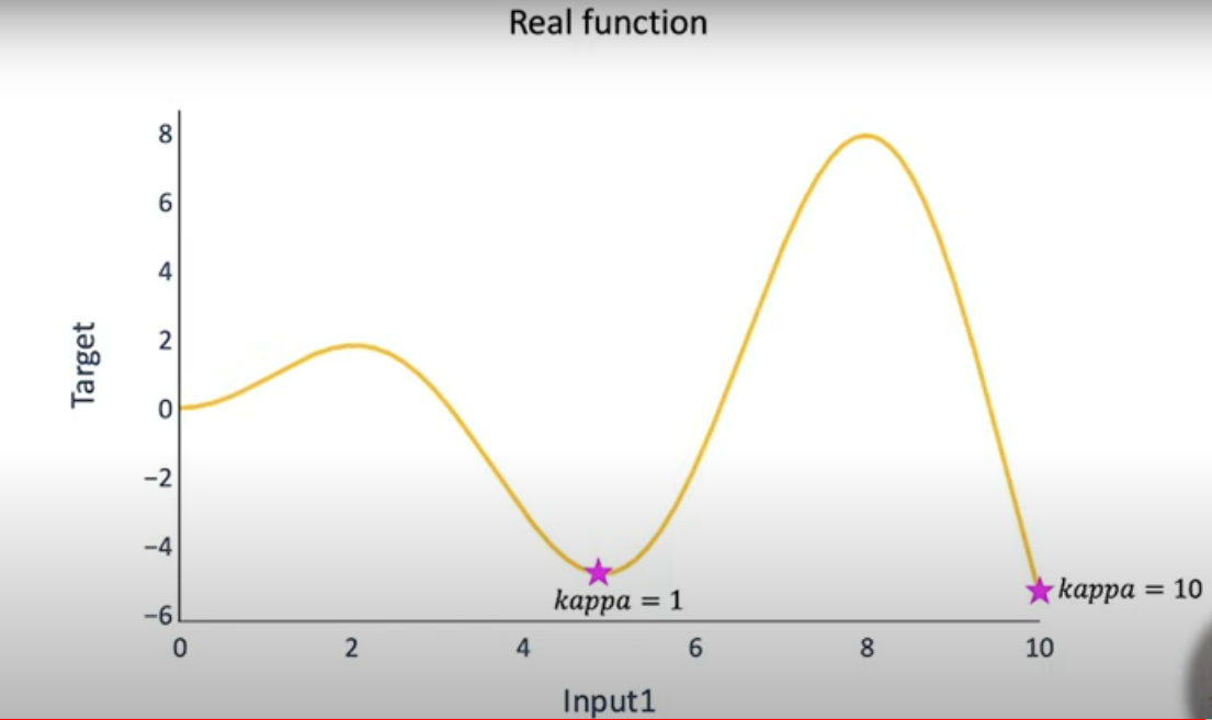
Note that in the above graph, when the value of the hyperparameter is 10, it gives the global minimum whereas when its value is 1, it only provides the local minimum. Hence, the hyperparameter chosen plays an important role because it gives the optimum point. This minimum, in turn, is a local minimum or the global minimum is the real challenge here.
Hyperparameter Tuning using Bayesian Optimization
Implementation is carried out using hyperopt package.
from hyperopt import hp,fmin,tpe,STATUS_OK,Trials
We then specify the list of values for our parameters just like how we did in GridSearchCV and RandomizedSearchCV.
space = {'criterion': hp.choice('criterion', ['entropy', 'gini']),
        'max_depth': hp.quniform('max_depth', 10, 1200, 10),
        'max_features': hp.choice('max_features', ['auto', 'sqrt','log2', None]),
        'min_samples_leaf': hp.uniform('min_samples_leaf', 0, 0.5),
        'min_samples_split' : hp.uniform ('min_samples_split', 0, 1),
        'n_estimators' : hp.choice('n_estimators', [10, 50, 300, 750, 1200,1300,1500])
    }
Next, we must define the objective function. This is something new in Bayesian Optimization and we had not done this in any of the techniques discussed so far.
def objective(space):
    model = RandomForestClassifier(criterion = space['criterion'], max_depth = space['max_depth'],
                                 max_features = space['max_features'],
                                 min_samples_leaf = space['min_samples_leaf'],
                                 min_samples_split = space['min_samples_split'],
                                 n_estimators = space['n_estimators'],
                                 )
    #5 times cross validation fives 5 accuracies=>mean of these accuracies will be considered
    accuracy = cross_val_score(model, X_train, y_train, cv = 5).mean()
    # We aim to maximize accuracy, therefore we return it as a negative value
    return {'loss': -accuracy, 'status': STATUS_OK }
Now it’s time to find the optimal values for these parameters using the Bayes opt.
from sklearn.model_selection import cross_val_score
trials = Trials()
best = fmin(fn= objective,
            space= space,
            algo= tpe.suggest,
            max_evals = 80,
            trials= trials)
The variable named ‘best’ has the optimal or best values. If you print it, you will get the following output:
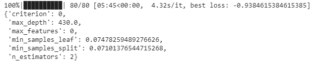
The values of the parameters criterion,max_features, and n_estimators are not the actual values; instead, they refer to the indices in the corresponding dictionaries. So, we must decode them to find out the actual optimal values of these parameters given by Bayes opt:
crit = {0: 'entropy', 1: 'gini'}
feat = {0: 'auto', 1: 'sqrt', 2: 'log2', 3: None}
est = {0: 10, 1: 50, 2: 300, 3: 750, 4: 1200,5:1300,6:1500}
print(crit[best['criterion']])
print(feat[best['max_features']])
print(est[best['n_estimators']])

Now, let’s re-train the model and predict with this model in order to check the performance of the new model:
trainedforest = RandomForestClassifier(criterion = crit[best['criterion']], max_depth = best['max_depth'],
                                       max_features = feat[best['max_features']],
                                       min_samples_leaf = best['min_samples_leaf'],
                                       min_samples_split = best['min_samples_split'],
                                       n_estimators = est[best['n_estimators']]).fit(X_train,y_train)
predictionforest = trainedforest.predict(X_test)
print(confusion_matrix(y_test,predictionforest))
print(accuracy_score(y_test,predictionforest))
print(classification_report(y_test,predictionforest))
What is TPOT Classifier?
TPOT stands for Tree-Based Pipeline Optimization Tool. It is used to automate Machine learning(AutoML). As the name suggests, it internally represents pipelines in the form of flexible ‘trees’.Its goal is to solve a given ML problem by automatically selecting one of the pipelines already available. Furthermore, it selects a pipeline among many based on its accuracy.
Genetic Programming(Genetic Algorithm)
It is based on the idea of ‘survival of the fittest. The popular theory proposed by Charles Darwin, states that only the best fit species will survive. Hence, the aim of our biological system is to pass on the best quality of parents to their children and thereby the best genes keep on getting transferred from a generation to its subsequent generations.
Similarly, Genetic programming is a hyperparameter optimization technique aiming to find the optimal solution from the given population. It is widely used to solve highly complex problems with wider search space and cannot be solved using the usual algorithms.
Phenotype refers to the raw and noisy inputs. Genotype, on the other hand, refers to fine and processed inputs. A phenotype has to thus be encoded to genotype and genotype can also be decoded to get phenotype back.
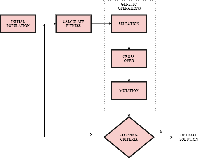
Initial Population:
The initial population must be as diverse as possible. More the diversity, the better will the performance of the algorithm be. For example, if you train your model to classify only black cats as cats, it will not work well on the images of golden cats because it has never seen golden cats before! That’s why diversity is important.
Fitness function:
The most stable output is given by the fitness function. Fitness is a measure of how relevant the prediction of the model is, to the true output. The fitness function is applied to all the values of the population.
Genetic operations:
1. Selection:
It is proportional to the fitness function. Here, the best parents having high values of fitness function will be selected. Generally, two parents are chosen to create a new population using cross-over and mutation.
2. Cross-over and Mutation:
The aim of cross-over and mutation is to generate a new population that takes us closer to the desired output for which their fitness values should be better than that of their previous generation.
There are several techniques of cross-over. For example, consider 2 words:horse and zebra.Say we must swap alphabet after 3rd position of the two words to get a new generation, then we will get the offsprings as horra and zebse respectively.
If our output is cake and a new generation results in the offsprings-bake, make and take, we can stop here as the fitness value of all the offsprings is the same and is equal to 4(as ‘ake’ is common in bake, make and take). Otherwise, if the fitness value decreases, we must backtrack and select parents with higher fitness values, as shown in the above flowchart. Cross-over should be repeated until an endpoint or, in other words, until convergence is reached.
Hyperparameter Optimization using TPOT
It is implemented using the tpot package. So, let’s go ahead and install it, in the first place:
!pip install tpot
Next, create an instance of the TPOTClassifier and obtain the optimal values for the parameters.
from tpot import TPOTClassifier
tpot_classifier = TPOTClassifier(generations= 5, population_size= 24, offspring_size= 12,
                                 verbosity= 2, early_stop= 12,
                                 config_dict={'sklearn.ensemble.RandomForestClassifier': param},
                                 cv = 4, scoring = 'accuracy')
tpot_classifier.fit(X_train,y_train)

As we have specified 5 generations, after running the 5th generation, the best pipeline’s values are displayed as shown in the above output. These are the required optimal values.
We then proceed to create a model with the optimal values as given by the TPOT technique.
rf_tpop=RandomForestClassifier(criterion='entropy', max_depth=120, max_features='auto', min_samples_leaf=2, min_samples_split=2, n_estimators=1400
                               )
rf_tpop.fit(X_train,y_train)
Now, it’s time to predict using the new model and thus check its performance as we did in the earlier techniques discussed so far.
predictionforest = rf_tpop.predict(X_test)
print(confusion_matrix(y_test,predictionforest))
print(accuracy_score(y_test,predictionforest))
print(classification_report(y_test,predictionforest))
acc = accuracy_score(y_test,predictionforest)
What is Optuna?
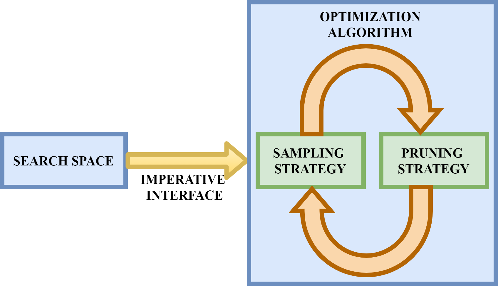
Optuna’s optimization algorithm ensures effective optimization using the following two components:
1. Sampling Strategy
2. Pruning Strategy
1. Sampling Strategy:
It tells us how to select the next hyperparameter and how to decide the next configuration using the previous history represented by Bayesian Optimization. A few examples include random search and CMA-ES which is a type of genetic algorithm.
We can also define our own sampling algorithm!!!
2. Pruning Strategy:
It detects the unpromising trials with the help of the intermediate learning curve. It performs early stopping of under-performing trials.
Hyperparameter Tuning using Optuna
It is implemented using the optuna package in Python.So, firstly, let us go ahead and install it:
!pip install optuna
Note that I have been using the exclamatory mark before the pip command as I have implemented all the code on Google Colab. If you are executing the above command in Google Colab or on Jupyter notebook, only then prefix the ‘!’ before pip in the above command.
Steps:
1. Define the objective function to minimize or maximize
2. Get hyperparameters with the suggest method
3. Run the search using study.optimize()
Steps 1 and 2:
import optuna
import sklearn.svm
def objective(trial):
    classifier = trial.suggest_categorical('classifier', ['RandomForest', 'SVC'])
    if classifier == 'RandomForest':
        n_estimators = trial.suggest_int('n_estimators', 200, 2000,10)
        max_depth = int(trial.suggest_float('max_depth', 10, 100, log=True))
        clf = sklearn.ensemble.RandomForestClassifier(
            n_estimators=n_estimators, max_depth=max_depth)
    else:
        c = trial.suggest_float('svc_c', 1e-10, 1e10, log=True)
        clf = sklearn.svm.SVC(C=c, gamma='auto')
    return sklearn.model_selection.cross_val_score(
        clf,X_train,y_train, n_jobs=-1, cv=3).mean()
Here, observe that we also want the Optuna technique to optimize between RandomForestClassifier and SVC. They suggest a method, as shown in the above code, has been used to achieve the same.
Step-3:
study = optuna.create_study(direction='maximize')
study.optimize(objective, n_trials=100)
trial = study.best_trial
print('Accuracy: {}'.format(trial.value))
print("Best hyperparameters: {}".format(trial.params))
Now, we set off to get the best parameters given by the Optuna technique.
study.best_params
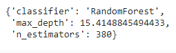
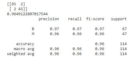
We should now re-train our RFClassifier with these optimal values and predict using it in order to check its performance.
rf=RandomForestClassifier(n_estimators=380,max_depth=15.4148845494433)
rf.fit(X_train,y_train)
y_pred=rf.predict(X_test)
print(confusion_matrix(y_test,y_pred))
print(accuracy_score(y_test,y_pred))
print(classification_report(y_test,y_pred))
Results
In this section, let’s finally compare the performances of all the models given by each of the hyperparameter optimization techniques discussed in this blog.
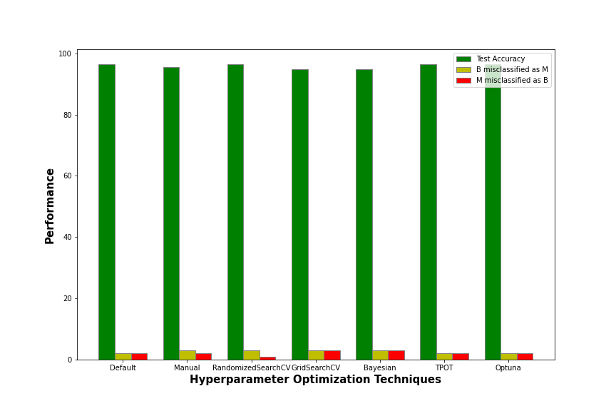
The above bar graph gives the test accuracy and the number of misclassifications, for both the categories, of each of the hyperparameter tuning techniques which we implemented. The test accuracy is nothing but the accuracy score of the model on the test dataset. It is denoted by the dark green bar. All such bars are tall which implies that all the models show good test accuracies!
‘B misclassified as M’ refers to the number of samples which are actually benign(B) but were misclassified by the model as malignant(M). It is denoted by the yellow bar.’M misclassified as B’ refers to the number of samples which are actually malignant(M) but were misclassified as benign(B). It is denoted by the red bar especially to indicate that this type of misclassification is dangerous. They can be noted in the confusion matrix as follows:
|
|
|
|
|
|
|
|
|
Thus, the best model is the one with the minimum number of dangerous misclassifications. Misclassifying M as B is dangerous because the patient is actually suffering from a harmful stage of breast cancer and will miss out on the important treatments required, as she was classified to be benign(B) which is a less harmful stage.
The models given by Bayesian and GridSearchCV optimization techniques are around 94.73% accurate but have 3 dangerous misclassifications. Coming to the model given by manual tuning, it shows an intermediate performance with around 95% accuracy. However, even in this case, the number of dangerous misclassifications is 2 which is also intermediate.
Finally, let’s talk about the models provided by the default model with default parameter values, RandomizedSearchCV, TPOT Classifier, and Optuna all of which perform the best, exhibiting around 96.49% accuracy. However, the model provided by RandomizedSearchCV’s optimal values outsmarts the rest with a comparatively lesser number of dangerous misclassifications. It has only 1 dangerous misclassification!
Therefore, the optimal values which are given by RandomizedSearchCV suit the best on our dataset, and thus RandomizedSearchCV is the best hyperparameter optimization technique for this problem. However, it will, of course, vary among datasets. So, every time, we must experiment with several hyperparameter tuning techniques before jumping to a conclusion.
You can get the entire code from here.
Hope you enjoyed reading my article.
Thank You.
References
1. All hyperparameter tuning techniques-implementation
2.GridSearchCV and RandomizedSearchCV-Theory
3. Bayesian optimization-Theory
About Me
I am Nithyashree V, a final year BTech Computer Science and Engineering student. I love learning such cool technologies and putting them into practice, especially observing how they help us solve society’s challenging problems. My areas of interest include Artificial Intelligence, Data Science, and Natural Language Processing.
You can read my other articles on Analytics Vidhya from here.
You can find me on LinkedIn from here.
The media shown in this article are not owned by Analytics Vidhya and are used at the Author’s discretion.


