This article was published as a part of the Data Science Blogathon
Convolutional neural networks, also called ConvNets, were first introduced in the 1980s by Yann LeCun, a computer science researcher who worked in the background. LeCun built on the work of Kunihiko Fukushima, a Japanese scientist, a basic network for image recognition.
The old version of CNN, called LeNet (after LeCun), can see handwritten digits. CNN helps find pin codes from postal. But despite their expertise, ConvNets stayed close to computer vision and artificial intelligence because they faced a major problem: They could not scale much. CNN’s require a lot of data and integrate resources to work well for large images.
At the time, this method was only applicable to low-resolution images. Pytorch is a library that can do deep learning operations. We can use this to perform Convolutional neural networks. Convolutional neural networks contain many layers of artificial neurons. Synthetic neurons, complex simulations of biological counterparts, are mathematical functions that calculate the weighted mass of multiple inputs and product value activation.
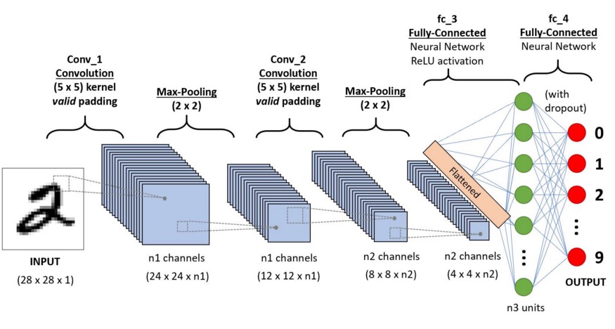
The above image shows us a CNN model that takes in a digit-like image of 2 and gives us the result of what digit was shown in the image as a number. We will discuss in detail how we get this in this article.
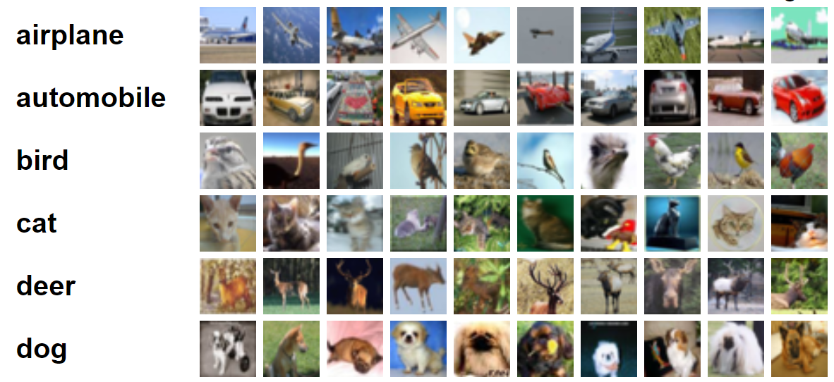
CIFAR-10 is a dataset that has a collection of images of 10 different classes. This dataset is widely used for research purposes to test different machine learning models and especially for computer vision problems. In this article, we will try to build a Neural network model using Pytorch and test it on the CIFAR-10 dataset to check what accuracy of prediction can be obtained.
import numpy as np
import pandas as pd
import torch
import torch.nn.functional as F
from torchvision import datasets,transforms
from torch import nn
import matplotlib.pyplot as plt
import numpy as np
import seaborn as sns
#from tqdm.notebook import tqdm
from tqdm import tqdm
In this step, we import the required libraries. We can see we use NumPy for numerical operations and pandas for data frame operations. The torch library is used to import Pytorch.
Pytorch has an nn component that is used for the abstraction of machine learning operations and functions. This is imported as F. The torchvision library is used so that we can import the CIFAR-10 dataset. This library has many image datasets and is widely used for research. The transforms can be imported so that we can resize the image to equal size for all the images. The tqdm is used so that we can keep track of the progress during training and is used for visualization.
Once we read the dataset we can see various labels like the frog, truck, deer, automobile, etc.
print("Number of points:",trainData.shape[0])
print("Number of features:",trainData.shape[1])
print("Features:",trainData.columns.values)
print("Number of Unique Values")
for col in trainData:
    print(col,":",len(trainData[col].unique()))
plt.figure(figsize=(12,8))
Output:
Number of points: 50000
Number of features: 2
Features: ['id' 'label']
Number of Unique Values
id : 50000
label : 10
In this step, we analyze the dataset and see that our train data has around 50000 rows with their id and associated label. There is a total of 10 classes as in the name CIFAR-10.
from torch.utils.data import random_split
val_size = 5000
train_size = len(dataset) - val_size

train_ds, val_ds = random_split(dataset, [train_size, val_size])
len(train_ds), len(val_ds)
This step is the same as the training step, but we want to split the data into train and validation sets.
(45000, 5000)
from torch.utils.data.dataloader import DataLoader

batch_size=64
train_dl = DataLoader(train_ds, batch_size, shuffle=True, num_workers=4, pin_memory=True)
val_dl = DataLoader(val_ds, batch_size, num_workers=4, pin_memory=True)
The torch.utils have a data loader that can help us load the required data bypassing various params like worker number or batch size.
@torch.no_grad()
def accuracy(outputs, labels):
    _, preds = torch.max(outputs, dim=1)
    return torch.tensor(torch.sum(preds == labels).item() / len(preds))

class ImageClassificationBase(nn.Module):
    def training_step(self, batch):
        images, labels = batch
        out = self(images)                  # Generate predictions
        loss = F.cross_entropy(out, labels) # Calculate loss
        accu = accuracy(out,labels)
        return loss,accu

    def validation_step(self, batch):
        images, labels = batch
        out = self(images)                    # Generate predictions
        loss = F.cross_entropy(out, labels)   # Calculate loss
        acc = accuracy(out, labels)           # Calculate accuracy
        return {'Loss': loss.detach(), 'Accuracy': acc}

    def validation_epoch_end(self, outputs):
        batch_losses = [x['Loss'] for x in outputs]
        epoch_loss = torch.stack(batch_losses).mean()   # Combine losses
        batch_accs = [x['Accuracy'] for x in outputs]
        epoch_acc = torch.stack(batch_accs).mean()      # Combine accuracies
        return {'Loss': epoch_loss.item(), 'Accuracy': epoch_acc.item()}

    def epoch_end(self, epoch, result):
        print("Epoch :",epoch + 1)
        print(f'Train Accuracy:{result["train_accuracy"]*100:.2f}% Validation Accuracy:{result["Accuracy"]*100:.2f}%')
        print(f'Train Loss:{result["train_loss"]:.4f} Validation Loss:{result["Loss"]:.4f}')
As we can see here we have used class implementation of ImageClassification and it takes one parameter that is nn.Module. Within this class, we can implement the various functions or various steps like training, validation, etc. The functions here are simple python implementations.
The training step takes images and labels in batches. we use cross-entropy for loss function and calculate the loss and return the loss. This is similar to the validation step as we can see in the function. The epoch ends combine losses and accuracies and finally, we print the accuracies and losses.
class Cifar10CnnModel(ImageClassificationBase):
    def __init__(self):
        super().__init__()
        self.network = nn.Sequential(
            nn.Conv2d(3, 32, kernel_size=3, padding=1),
            nn.ReLU(),
            nn.Conv2d(32, 64, kernel_size=3, stride=1, padding=1),
            nn.ReLU(),
            nn.MaxPool2d(2, 2), # output: 64 x 16 x 16
            nn.BatchNorm2d(64),

            nn.Conv2d(64, 128, kernel_size=3, stride=1, padding=1),
            nn.ReLU(),
            nn.Conv2d(128, 128, kernel_size=3, stride=1, padding=1),
            nn.ReLU(),
            nn.MaxPool2d(2, 2), # output: 128 x 8 x 8
            nn.BatchNorm2d(128),

            nn.Conv2d(128, 256, kernel_size=3, stride=1, padding=1),
            nn.ReLU(),
            nn.Conv2d(256, 256, kernel_size=3, stride=1, padding=1),
            nn.ReLU(),
            nn.MaxPool2d(2, 2), # output: 256 x 4 x 4
            nn.BatchNorm2d(256),

            nn.Flatten(),
            nn.Linear(256*4*4, 1024),
            nn.ReLU(),
            nn.Linear(1024, 512),
            nn.ReLU(),
            nn.Linear(512, 10))

    def forward(self, xb):
        return self.network(xb)
This is the most important part of neural network implementation. Throughout, we use the nn module we imported from torch. As we can see in the first line, the Conv2d is a module that helps implement a convolutional neural network. The first parameter 3 here represents that the image is colored and in RGB format. If it was a grayscale image we would have gone for 1.
32 is the size of the initial output channel and when we go for the next conv2d layer we would have this 32 as the input channel and 64 as the output channel.
The 3rd parameter in the first line is called kernel size and it helps us take care of the filters used. Padding operation is the last parameter.
The convolution operation is connected to an activation layer and Relu here. After two Conv2d layers, we have a max-pooling operation of size 2 * 2. The value coming out from this is batch normalized for stability and to avoid internal covariate shift. These operations are repeated with more layers to deeper the network and reduce the size. Finally, we flatten the layer so that we can build a linear layer to map the values to 10 values. The probability of each neuron of these 10 neurons will determine which class a particular image belongs to based on the maximum probability.
@torch.no_grad()
def evaluate(model, data_loader):
    model.eval()
    outputs = [model.validation_step(batch) for batch in data_loader]
    return model.validation_epoch_end(outputs)

def fit(model, train_loader, val_loader,epochs=10,learning_rate=0.001):
    best_valid = None
    history = []
    optimizer = torch.optim.Adam(model.parameters(), learning_rate,weight_decay=0.0005)
    for epoch in range(epochs):
        # Training Phase
        model.train()
        train_losses = []
        train_accuracy = []
        for batch in tqdm(train_loader):
            loss,accu = model.training_step(batch)
            train_losses.append(loss)
            train_accuracy.append(accu)
            loss.backward()
            optimizer.step()
            optimizer.zero_grad()
        # Validation phase
        result = evaluate(model, val_loader)
        result['train_loss'] = torch.stack(train_losses).mean().item()
        result['train_accuracy'] = torch.stack(train_accuracy).mean().item()
        model.epoch_end(epoch, result)
        if(best_valid == None or best_valid<result['Accuracy']):
            best_valid=result['Accuracy']
            torch.save(model.state_dict(), 'cifar10-cnn.pth')
        history.append(result)
    return history
history = fit(model, train_dl, val_dl)
This is a basic step to train our model to get the required result. the fit function here will fit the train and Val data with the model we created. The fit function takes initially a list called history that takes care of the iteration data of every epoch. We run a for loop so that we can iterate over each epoch. For each batch, we make sure we show the progress using tqdm. We call the training step we implemented before and calculate accuracy and loss. The go for backward propagation and run optimizer which we defined earlier. Once we do this we keep track of our list and the functions help us print the details and progress.
The evaluate function, on the other hand, uses the eval function, and for each step, we take the batch loaded from the data loader, and output is calculated. The value then is passed to the validation epoch end we defined earlier and the respective value is returned.
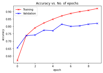
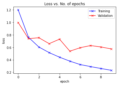
In this step, we will visualize the accuracy vs each epoch. We can observe that as the epoch increase the accuracy of the system keeps increasing and similarly the loss keeps decreasing. The red line here indicates training data progress and blue for the validation. We can see that there has been a good amount of overfitting in our results as the training data is quite outperforming the validation result and similarly in case of loss. After 10 epochs, the train data seems to bypass 90% accuracy but has a loss of around 0.5. The test data comes around 81% and the losses are near 0.2.
def plot_accuracies(history):
    Validation_accuracies = [x['Accuracy'] for x in history]
    Training_Accuracies = [x['train_accuracy'] for x in history]
    plt.plot(Training_Accuracies, '-rx')
    plt.plot(Validation_accuracies, '-bx')
    plt.xlabel('epoch')
    plt.ylabel('accuracy')
    plt.legend(['Training', 'Validation'])
    plt.title('Accuracy vs. No. of epochs');
plot_accuracies(history)
def plot_losses(history):
    train_losses = [x.get('train_loss') for x in history]
    val_losses = [x['Loss'] for x in history]
    plt.plot(train_losses, '-bx')
    plt.plot(val_losses, '-rx')
    plt.xlabel('epoch')
    plt.ylabel('loss')
    plt.legend(['Training', 'Validation'])
    plt.title('Loss vs. No. of epochs');
plot_losses(history)
In the final step, we want to check the accuracy of the system. The transform parameter helps us get the data and transform them to tensors so that we can use it to input for testing. Here we load the data in batches using the device data loader and the device parameter can be tuned to get the testing done in CPU or GPU. Finally, we use our evaluate function to evaluate our model against the test data and as per the functions we defined above we will get the accuracy as result.
test_dataset = ImageFolder(data_dir+'/test', transform=ToTensor())
test_loader = DeviceDataLoader(DataLoader(test_dataset, batch_size), device)
result = evaluate(final_model, test_loader)
print(f'Test Accuracy:{result["Accuracy"]*100:.2f}%')
Test Accuracy:81.07%
We can see that we end up with an accuracy of 81.07%.
Image:https://unsplash.com/photos/5L0R8ZqPZHk
About Me: I am a Research Student interested in the field of Deep Learning and Natural Language Processing and currently pursuing post-graduation in Artificial Intelligence.
Feel free to connect with me on:
Lorem ipsum dolor sit amet, consectetur adipiscing elit,


