This article was published as a part of the Data Science Blogathon
Introduction to Machine Learning
Before jumping to Supervised Machine Learning, let’s understand a bit about Machine Learning. Machine Learning is an enticing field of study that leverages mathematics to solve complex real-world problems. The traditional algorithms need us to give a set of data and rules to the system and produce answers based on that. The machine learning algorithms take in data and answers and produce rules based on data and answers.
The data and answers refer to the features and target of the data and the rules produced refer to the trained model. Machine learning is used in a variety of industries like Agriculture, Software, Automobiles, Hospitals, and Healthcare.
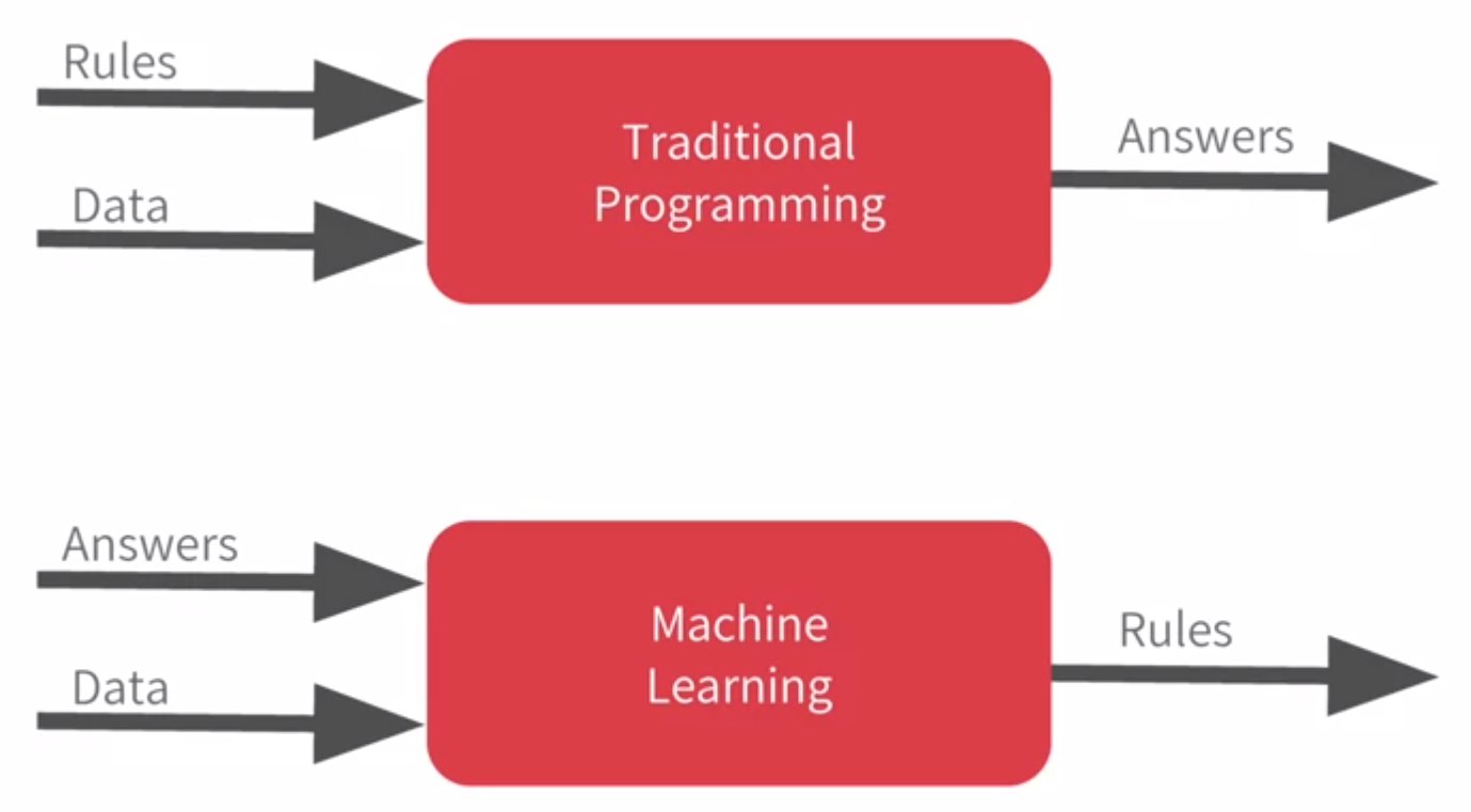
Image 1
Table of Contents
- Types of learning
- Supervised learning
- Unsupervised learning
- Reinforcement learning
- Approaching a Supervised Machine Learning Problem
- Data Preprocessing
- Handling Imbalanced Data
- Data Cleaning
- Data Transformation
- Data Reduction
- Data Modeling
- Regression algorithms
- Classification algorithms
- Performance Metrics
- Classification metrics
- Regression metrics
- Solving a Classification problem using Kaggle’s Titanic data
- Deployment
- Flask
- Docker
Types of Learning
- Supervised Learning
- Unsupervised Learning
- Reinforcement Learning
1. Supervised Learning
Supervised learning is a type of learning that requires features and targets in data. For example, to predict a house price the feature would be the house price column and the features would look like the number of bedrooms, square feet, location, and etc.
The supervised model attempts to learn the relationship between the features and the target and leverage the model to predict the unseen data. The target is necessary to learn the X->Y mapping in the data.
Supervised learning can be further classified into,
1.1 Regression
1.2 Classification
1.1 Regression
Regression is a type of supervised machine learning in which the target values contain continuous data. Examples of continuous data include 1.2, 3.1, and etc.
Linear regression attempts to find the optimal parameters for the model by the concept called correlation. The following are the assumptions of linear regression
- Linearity
- No Multicollinearity
- Normality
- Homoscedasticity
- No autocorrelation of the residuals
Widely used Regression algorithms include,
- Linear Regression
- Random Forest Regressor
- Gradient Boosting Regressor
- Polynomial Regression
- XGBoost Regressor
1.2 Classification
Classification is a type of supervised machine learning in which the target values contain discrete data or categorical data. Examples of categorical data include red, green, and etc. The target classes can be binary or multi-class.
A binary target refers to having only two unique classes in the target variable but in the multi-class target refers to having more than two unique classes in the target column.
Widely used Classification algorithms include,
- Logistic Regression
- Decision Trees
- Random Forest
- SVM
- XGBoost Classifier
2. Unsupervised Learning
Unsupervised learning is a type of learning that finds the underlying pattern in the provided data. Clustering techniques include K-Means attempt to find similar data and attempts to group it together around the centroids.
Clustering is very useful in segmenting customers and identifying similar customer behaviors. Clustering techniques are employed to detect anomalies in the dataset.
The types of unsupervised algorithms include,
- K-Means
- K-Medoids
- The DBSCAN algorithm
3. Reinforcement Learning
Reinforcement learning is a field of study in which an agent interacts with the environment and takes action based on the interaction. The agent receives rewards based on the action it has performed.
The types of reinforcement algorithms include,
- Q-Learning
- Multi-armed bandits
In this post, we are going to focus on supervised learning and the techniques to approach the problem and deploy it using flask and docker.
Approaching a Supervised Machine Learning Problem
Before feeding the data to the model it is very important to preprocess the data. The model follows a simple rule “Garbage in, garbage out”, the quality of the model depends on the quality of the data that you feed in. So, data preprocessing plays an important role in approaching the machine learning problem.
Data Preprocessing
Data preprocessing is a process that needs to be carried out in order to produce high-quality solutions. 80% of the work carried out in the machine learning pipeline would be data preprocessing.
The real-world data are noisy, inconsistent, and incomplete. The model couldn’t handle all these inherent and vicious attributes of data. Noisy data refers to the random errors, and inconsistent data refers to the inconsistent entries in the data, incomplete data refers to the data that is not available.
The data preprocessing consists of three stages,
- Handling Imbalanced Data
- Data Cleaning
- Data Transformation
- Data Reduction
Import required data,
import pandas as pd
TRAIN_DATA_PATH = 'https://raw.githubusercontent.com/agconti/kaggle-titanic/master/data/train.csv'
TEST_DATA_PATH = 'https://raw.githubusercontent.com/agconti/kaggle-titanic/master/data/test.csv'
TARGET_NAME = 'Survived'
train_data = pd.read_csv(TRAIN_DATA_PATH)
test_data = pd.read_csv(TEST_DATA_PATH)
# x_train = features, y_train = target
train_data = pd.read_csv(TRAIN_DATA_PATH)
test_data = pd.read_csv(TEST_DATA_PATH)
x_train, y_train = train_data.drop([TARGET_NAME, 'PassengerId'], axis=1), train_data[TARGET_NAME]
x_test = test_data
1. Handling Imbalanced Data
A data is said to be imbalanced if the class distributions of the target are not proportionate. There are a lot of ways to handle imbalanced data, use different metrics like F1 score, ROC-AUC score instead of accuracy.
An alternative process is to use random oversampling or undersampling. Oversampling or undersampling can be done using the Imblearn package in python. Having imbalanced data gives you a false notion about the accuracy, when you train imbalanced data you would get high accuracy thereby misleading you.
Execute the following command to install the package,
pip install imblearn
The following code demonstrates the usage of random undersampling,
from imblearn.under_sampling import RandomUnderSampler
undersample = RandomUnderSampler(sampling_strategy='majority')
x_train_undersampled, y_train_undersampled = oversample.fit_resample(x_train, y_train)
SMOTE and ADASYN are other techniques to oversample the data.
2. Data Cleaning
Missing value imputation is a part of data cleaning. Missing value imputation is a process of filling in the missing values in the data. Missing value imputation for numeric data differs from categoric data.
For numeric data, we can use techniques like mean imputation, median imputation and for categoric data, we can use techniques like mode imputation. Other imputation techniques are KNN, MissForest, and Linear Regression to impute the data.
Median imputation
Median is the middlemost value in the data. The mean imputation is highly prone to be affected by the influence of outliers.
Mode imputation
Mode is the value that occurs more in the data. Mode imputation can be used to impute categorical data.
from sklearn.impute import SimpleImputer
si_median = SimpleImputer(strategy="median")
si_mode = SimpleImputer(strategy="most_frequent")
numeric_data = x_train.select_dtypes('number')
categoric_data = x_train.select_dtypes(exclude='number')
# median imputation
numeric_data_imputed = pd.DataFrame(
    si_median.fit_transform(numeric_data.copy()),
    columns=numeric_data.columns,
    index=numeric_data.index
)
# mode imputation
categoric_data_imputed = pd.DataFrame(
    si_mode.fit_transform(categoric_data.copy()),
    columns=categoric_data.columns,
    index=categoric_data.index
)
# concatenating numeric and categoric data
X_train_imputed = pd.concat(
    [numeric_data_imputed, categoric_data_imputed],
    axis=1
)
In the above code, we used SimpleImputer to impute the numeric columns with the median of those columns and impute categoric columns with the mode of those columns. The method named select_dtypes is used to select the data with the provided data type, in our case we selected ‘number’ which would select all the numerical data.
3. Data Transformation
Data transformation is the process of transforming the data in order to increase the model performance. Widely used data transformation techniques are categorical encoding, standardization, and normalization.
Representing the data on a different scale might reduce the effect of outliers in the data. For example, let us say that a column in the data is highly right-skewed. In order to reduce the skewness, we need to transform the data using log transformation. By doing so, the data produced would be without skewness and with normal distribution.
1. Categorical encoding
Categorical encoding is the process of converting categorical data into numeric data. The purpose of categorical encoding is that the models can’t handle string data directly so we need to represent the string data in a numerical format. Even though we are representing the data in the numerical format the model handles it as a discrete variable.
There are many types of categorical encoding available like label encoding, target encoding, frequency encoding, m-estimate encoding, and one-hot encoding. In this post, we are going to see about label encoding, frequency encoding, and target encoding.
1.1 Label encoding
Label encoding directly assigns a number to the category and replaces that category with that number. It finds out the unique categories in the data and assigns a number to the category. We can use scikit-learn’s LabelEncoder to perform label encoding.
1.2 Frequency encoding
Frequency encoding maps the frequencies of each category to the category values. For example, the column contains the value ‘red’ with a frequency of 5 and ‘green’ with a frequency of 7, then the value ‘red’ is replaced with 5 and the ‘green’ value is replaced with 7.
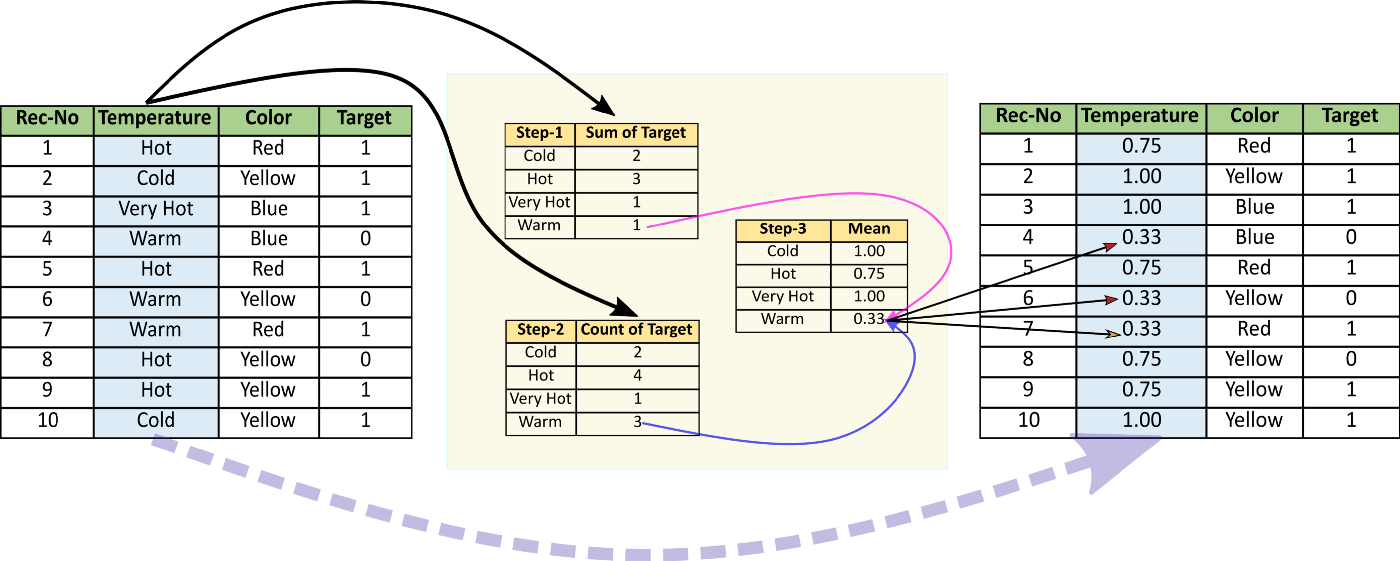
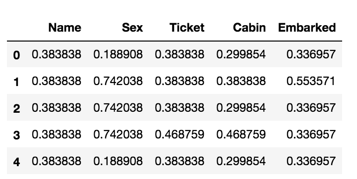
1.3 Target encoding
Target encoding maps the mean of the target with respect to the categories. Target encoding requires targets to encode the variables. We can make use of the category_encoders package to perform target encoding.
Installing category_encoders,
pip install category_encoders
from sklearn.preprocessing import LabelEncoder
from category_encoders import CountEncoder, TargetEncoder
label_encoder = LabelEncoder()
count_encoder = CountEncoder()
target_encoder = TargetEncoder()
# label encoding
c_data = categoric_data.copy()
for col in categoric_data.columns:
    c_data[col] = label_encoder.fit_transform(c_data[col])
c_data.head()
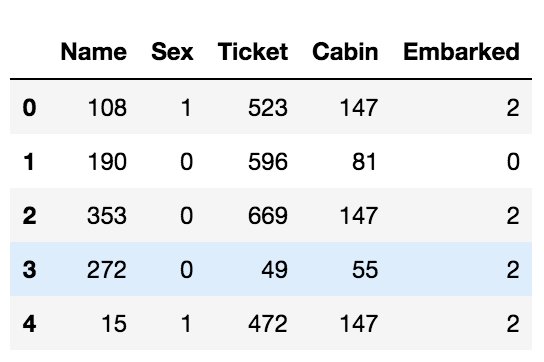
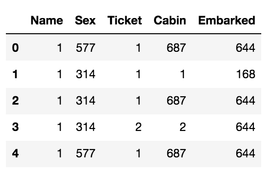
# frequency encoding
c_data = count_encoder.fit_transform(categoric_data.copy())
c_data.head()
# target encoding
c_data = target_encoder.fit_transform(categoric_data, y_train)
c_data.head()
2. Standardization
Standardization is the process of scaling the features such that the mean is 0 and the standard deviation is 1. The purpose of using standardization is to convert the data into similar scales and to make the training process faster in case if we used optimization techniques such as gradient descent and etc. Standardization would help us to improve the accuracy of the model.
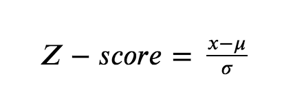
2.1 Z-Score
Z-Score is a widely used standardization technique. It simply subtracts the mean of the data from each data and divides it by the standard deviation of the data.
Author’s Jupyter Notebook
We can perform standardization using Sklearn’s StandardScaler class.
from sklearn.preprocessing import StandardScaler
scaler = StandardScaler()
x_train_scaled = scaler.fit_transform(x_train)
3. Normalization
Normalization is the process of scaling data such that it falls between a certain interval. For example, we can scale a feature such that the data it contains falls under 0 and 1.
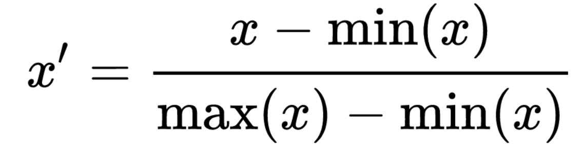
3.1 Min-max normalization
Min-max normalization is a widely used normalization technique. Min-max normalization utilizes the min and max of the feature to scale the data.
We can perform normalization using Sklearn’s MinMaxScaler class.
from sklearn.preprocessing import MinMaxScaler
scaler = MinMaxScaler()
x_train_scaled = scaler.fit_transform(x_train)
4. Data Reduction
Data reduction is the process of reducing the data along the column axis. We perform data reduction techniques to avoid the overfitting phenomenon. Overfitting is a phenomenon in which the model would show high performance in training but fails to generalize to the new unseen data.
One of the dimensionality reduction techniques is feature selection which discards a feature after looking at the importance of the feature statistically. There are a wide variety of feature selection techniques available like RFE (Recursive Feature Elimination), RFECV (Recursive Feature Elimination with Cross Validation), and Sequential Feature Selector.
RFE (Recursive Feature Elimination)
Recursive Feature Elimination is a type of wrapper feature selection that requires a model to find the importance of the feature. As the name says, It recursively eliminates the feature according to the importance of the feature.
The setback of using RFE is that we have to provide a number of features to select. To overcome this we can use RFECV which uses cross-validation to determine the number of features to select. In the code below, the x_train must be preprocessed before using it.
from sklearn.feature_selection import RFE
from sklearn.ensemble import RandomForestClassifier
estimator = RandomForestClassifier()
selector = RFE(estimator, n_features_to_select=5)
selector = selector.fit(x_train, y_train)
selector.support_
RFECV (Recursive Feature Elimination with Cross Validation)
Recursive Feature Elimination with Cross Validation is a type of wrapper feature selection that is very similar to RFE but eliminates the hyperparameter n_features_to_select.
It recursively eliminates the features and uses cross-validation to determine the number of features to select.
from sklearn.feature_selection import RFECV
from sklearn.ensemble import RandomForestClassifier
estimator = RandomForestClassifier()
selector = RFECV(estimator)
selector = selector.fit(x_train, y_train)
selector.n_features_
Data Modeling
Data modeling is the process of training a model that learns the relationship between the features and the target. A large amount of data is preferable because more the data more are the patterns to learn. The trained model is then used to predict the new unseen model. A highly complex and flexible model like Decision-Tree is more prone to overfit the data.
To avoid overfitting we can use ensemble methods. Bagging is the process of combining several weak models to produce an efficient model but the Boosting algorithms make use of several weak models and feed each of the weak model’s output to the next weak model thereby producing an efficient model.
An example of a bagging algorithm is the Random Forest algorithm and an example of a boosting algorithm is the Gradient Boosting algorithm. We can also use cross-validation techniques to select the best model.
Performance metrics for Supervised Machine Learning Model
Performance metrics are used to assess the quality of the trained model. In regression model training is referred to as learning the parameters of the model, so measuring the performance means, how well the model has learned the parameters. To know the performance we use cost functions that compare the predicted and actual values.
Regression and classification techniques require a separate set of metrics to analyze the performance of the model. Gradient descent, RMS Prop, and Adam are cost function optimization techniques to optimize the model. The gradient descent optimization algorithm finds the optimal parameters of the model by finding the error gradients. We can run the algorithm for many cycles until we arrive at a globally optimal solution.
Widely used Regression metrics
- Mean squared error
- Mean squared logarithmic error
- Mean absolute error
Widely used Classification metrics
- Accuracy score
- F1 score
- ROC-AUC score
- Log loss
Solving a Classification problem using Kaggle’s Titanic data
Before getting into solving the problem, let us have a look at what Flask is.
What is Flask

Flask is a web application framework written in python to build web applications and API architecture. In this post, we have utilized flask to develop an API for training and testing the titanic dataset.
Devolping an API using Flask
FlaskAndDocker
|—-> training.py
|—-> utils.py
|—-> requirements.txt
|—-> Dockerfile
The following code is in the module utils.py. The following code is used for frequency encoding, median and mode imputation, and robust scaling. All these are used for preprocessing.
import pandas as pd
from sklearn.base import TransformerMixin
from sklearn.metrics import accuracy_score
from sklearn.preprocessing import RobustScaler
model_path = "/FlaskAndDocker/model.pkl"
pipeline_path = '/FlaskAndDocker/pipeline.pkl'

TRAIN_DATA_PATH = 'https://raw.githubusercontent.com/agconti/kaggle-titanic/master/data/train.csv'
TEST_DATA_PATH = 'https://raw.githubusercontent.com/agconti/kaggle-titanic/master/data/test.csv'
TARGET_NAME = 'Survived'

class FrequencyEncoder(TransformerMixin):
"""
 Frequency Encoder that handles ties in
 encoding.

 """

 def __init__(self, handle_unknown):
self.handle_unknown = handle_unknown

@staticmethod
def _get_categoric_columns(data):
"""Return categoric column names"""

 data_dtypes_dict = dict(data.dtypes)

categorical_columns = [
k for k, v in data_dtypes_dict.items()
if v == 'object' or pd.api.types.is_categorical_dtype(v)
]

return categorical_columns

def fit(self, X, y=None):
"""
 Parameters
 ----------
 X : pandas.DataFrame
 y : ignored

 Returns
 -------
 self : object
 """

self.categorical_columns =
FrequencyEncoder._get_categoric_columns(X)

if len(self.categorical_columns) == 0:
return self

self.frequency_dict_ = {}
data_len = len(X)

for col in self.categorical_columns:
value_counts = X[col].value_counts()
self.frequency_dict_[col] = dict(value_counts/data_len)

return self

def transform(self, X):
"""
 Parameters
 ----------
 X : pandas.DataFrame
 y : ignored

 Returns
 -------
 ranked_data : pandas.DataFrame
 """

if len(self.categorical_columns) == 0:
return X

for col in self.categorical_columns:
"""Normalized during train"""
frequencies = self.frequency_dict_[col]
X.loc[:, col] = X[col].map(frequencies)
X[col].fillna(self.handle_unknown, inplace=True)

return X

class Imputer(TransformerMixin):
"""
 Median and Mode imputer

 """

 def __init__(self, strategy):
self.strategy = strategy

@staticmethod
def to_lowercase(x):
if pd.isnull(x):
return x
return x.lower()

def fit(self, X, y=None):
"""

 Parameters
 ----------
 X : pandas.DataFrame
 y : ignored

 Returns
 -------
 self : object
 """
if self.strategy == 'median':

self.numerical_columns = list(X.select_dtypes('number').columns)
self.median_dict_ = {}

if len(self.numerical_columns) == 0:
return self

for col in self.numerical_columns:
self.median_dict_[col] = X[col].median()

elif self.strategy == 'mode':

self.categorical_columns = list(X.select_dtypes('object').columns)
self.mode_dict_ = {}

if len(self.categorical_columns) == 0:
return self

for col in self.categorical_columns:
"""Lowercase and fit"""
X.loc[:, col] = X[col].map(Imputer.to_lowercase)
self.mode_dict_[col] = X[col].mode().iloc[0]

return self

def transform(self, X):
"""

 Parameters
 ----------
 X : pandas.DataFrame

 Returns
 -------
 X : pandas.DataFrame
 Imputed data
 """
if self.strategy == 'median':

if len(self.numerical_columns) == 0:
return X

for col in self.numerical_columns:
X[col].fillna(self.median_dict_[col], inplace=True)

elif self.strategy == 'mode':

if len(self.categorical_columns) == 0:
return X

for col in self.categorical_columns:
"""Lowercase and impute"""
X.loc[:, col] = X[col].map(Imputer.to_lowercase)
X[col].fillna(self.mode_dict_[col], inplace=True)

return X

class CustomRobustScaler(RobustScaler):

def __init__(self, **params):
super().__init__(**params)

def _get_original_data(self, X, scaled_data):

"""Concatenate numerical and
 categorical columns"""

 X_numeric_data = pd.DataFrame(
scaled_data,
columns=self.numerical_columns
)
X_remnant_data = X.drop(self.numerical_columns, axis=1)

X_original = pd.concat(
[
X_numeric_data.reset_index(drop=True),
X_remnant_data.reset_index(drop=True)
],
axis=1
)
X_original = X_original.sort_index(axis=1)

return X_original

def fit(self, X, y=None):
"""
 Parameters
 ----------
 X : pandas.DataFrame
 y : ignored

 Returns
 -------
 self : object
 """
self.numerical_columns = list(X.select_dtypes(['number']).columns)
print(f"Num COls: {self.numerical_columns}")

if len(self.numerical_columns) == 0:
"""No numerical columns detected"""
return self

X_numeric = X[self.numerical_columns]
super().fit(X_numeric)
return self

def transform(self, X):
"""
 Parameters
 ----------
 X : pandas.DataFrame

 Returns
 -------
 X_original : scaled data
 """

if len(self.numerical_columns) == 0:
return X

X_numeric = X[self.numerical_columns]
scaled_data = super().transform(X_numeric)

X_original = self._get_original_data(X, scaled_data)

return X_original

def fit_model(model, X, y):
model.fit(X, y)
y_pred = model.predict(X)
acc_score = accuracy_score(y, y_pred)
acc_dict = {
'model': model,
"model_name": model.__class__.__name__,
"accuracy": acc_score
}
return acc_dict
The following requirements should be available in the requirements.txt file
Flask==2.0.1
numpy==1.21.2
pandas==1.2.4
scikit_learn==1.0
The following code must be inside the training.py module
import pickle
from utils import *
from flask import Flask
from sklearn.pipeline import Pipeline
from sklearn.linear_model import LogisticRegression
from sklearn.ensemble import RandomForestClassifier
from sklearn.ensemble import GradientBoostingClassifier
app = Flask(__name__)

@app.route("/train_titanic")
def train_titanic():
train_data = pd.read_csv(TRAIN_DATA_PATH)

x_train, y_train = (
train_data.drop([TARGET_NAME, 'PassengerId'], axis=1),
train_data[TARGET_NAME]
)

data_len = x_train.shape[0]
median_imputer = Imputer('median')
mode_imputer = Imputer('mode')
robust_scaler = CustomRobustScaler()
frequency_encoder = FrequencyEncoder(handle_unknown=1 / data_len)

preprocessing_steps = [
'median_imputer', 'mode_imputer',
'robust_scaler', 'frequency_encoder',
]
preprocessing_instances = [
median_imputer, mode_imputer,
robust_scaler, frequency_encoder
]

pipeline_steps = list(zip(preprocessing_steps, preprocessing_instances))
pipeline = Pipeline(pipeline_steps)

# Preprocessing
x_train_preprocessed = pipeline.fit_transform(x_train.copy())

accuracy_list = []
models = [
LogisticRegression(),
GradientBoostingClassifier(),
RandomForestClassifier()
]

for model in models:
acc_dict = fit_model(model, x_train_preprocessed, y_train)
accuracy_list.append(acc_dict)

acc_df = pd.DataFrame(accuracy_list).sort_values("accuracy", ascending=False)
model = acc_df.iloc[0]['model']
accuracy = acc_df.iloc[0]['accuracy']

pickle.dump(model, open(model_path, 'wb'))
pickle.dump(pipeline, open(pipeline_path, 'wb'))

return {
"status": "success",
"selected_model": f"{model.__class__.__name__}",
"accuracy": f"{accuracy}",
}

@app.route("/test_titanic")
def test_titanic():
test_data = pd.read_csv(TEST_DATA_PATH)
x_test = test_data.drop("PassengerId", axis=1)

try:
model = pickle.load(open(model_path, 'rb'))
pipeline = pickle.load(open(pipeline_path, 'rb'))

except Exception as e:
print(f"Exception: {e}")
return {
'status': "failure",
"message": "Train the model first"
}

x_test_preprocessed = pipeline.transform(x_test)
predictions = model.predict(x_test_preprocessed)

return {
"status": "success",
"predictions": predictions.tolist()
}

if __name__ == "__main__":
app.run(host='0.0.0.0', port=8088)
How does the above code work?
First of all, the code defines a preprocessing pipeline, in our case, it is a pipeline that consists of Median imputation, Mode imputation, Robust Scaler, and Frequency encoding. The median imputer class imputes the missing values in the numerical columns with the median of those columns and the mode imputer imputes the missing values in categorical columns with the mode (the most frequent category) of those columns and Robust scaler standardizes the data such that the mean is zero and the standard deviation is one with a more robust way that is not influenced by the outliers and the frequency encoder encodes the categorical data by mapping the categories with the frequencies of those categories.
When the fit_transform method is invoked the above pipeline would be executed. At first, the pipeline code splits the data into numeric and categoric columns and applies appropriate preprocessing respectively. After performing/running a pipeline object we must pickle the pipeline object to utilize it for transforming the test data. The methodology used here to write preprocessors is also called the custom transformers, by taking advantage of the custom transformers you can give additional functionality to the data.
After running the pipeline and preprocessing the data we train different models on the preprocessed data and check the accuracy. We have used Logistic Regression, Gradient Boosting classifier, and Random Forest classifier to train. In our case, the Random forest classifier performed better with an accuracy of 98%.
After training the model, we have to pickle the model to predict it on the future data. Pickling is a serialization technique that persists the model’s state and behavior.
To run the code, execute the following command
python3 training.py
After running it you would get logs like,
Serving Flask app 'training' (lazy loading)
 * Environment: production
   WARNING: This is a development server. Do not use it in a production deployment.
   Use a production WSGI server instead.
 * Debug mode: off
 * Running on all addresses.
   WARNING: This is a development server. Do not use it in a production deployment.
 * Running on http://0.0.0.0:8088/ (Press CTRL+C to quit)Serving Flask app 'training' (lazy loading)
To train the model, hit the following URL in the browser, http://0.0.0.0:8088/train_titanic
You would get output like,
{
  "accuracy": "0.9831649831649831",
  "selected_model": "RandomForestClassifier",
  "status": "success"
}
To test the model, hit the following URL in the browser, http://0.0.0.0:8088/test_titanic
You would get output in the following format,
{
    "status": "success",
    "predictions": [0, 1, ......, 0]
}
Deployment of Supervised Machine Learning Model
Deploying a machine learning model is a very challenging task. Making the model’s predictions available to customers is called deployment.
Docker
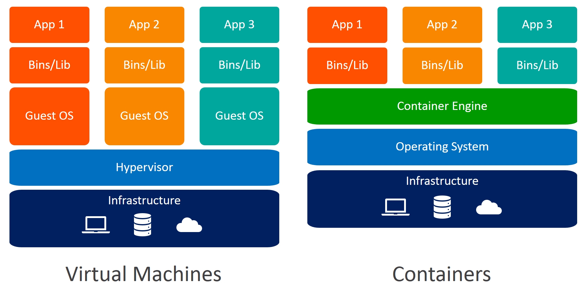
Docker is a containerization tool and an open-source platform that helps developers to build apps and deploy them. Docker can make an application run in an isolated environment. We can have many containers to run on a host using the same docker image. Containers don’t require an additional load of hypervisors as in VM and it can load in seconds and it can use much lesser resource than VMs.
Docker vs Virtual Machines
-
Docker is OS-level virtualization. VMs (Virtual Machines) are hardware-level virtualization.
- Docker boots faster. VM requires hypervisors which allocates resources.
- Creating a virtual machine takes a long time to start. Creating the containers requires much less time.
- The virtual machine needs additional resources. The docker doesn’t need more resources compared to VM.
- Virtual machine requires exclusive kernel for each VM. All the containers that are in docker use the host’s kernel.
There are three terminologies you need to know in Docker,
- Docker file
- Docker image
- Docker container
A Docker file is a blueprint of the docker image. The Docker file consists of instructions layer by layer for building an image. A docker image is a read-only template of the container. We can build even more layers on top of an image.
A running instance of a docker image is a docker container. You can create many containers based on a single docker image.
Dockerfile contents,
FROM ubuntu
ADD . /FlaskAndDocker
WORKDIR /FlaskAndDocker
ENV TZ=Asia/Kolkata
RUN ln -snf /usr/share/zoneinfo/$TZ /etc/localtime && echo $TZ > /etc/timezone
RUN apt-get update && apt-get install python3.6 -y && apt-get install python3-pip -y
RUN apt-get install vim -y
RUN pip3 install -r requirements.txt
CMD [“/bin/bash”]
-
The command ‘FROM ubuntu’ means that the ubuntu image is the base image, if there is no image found locally, the docker finds it from the docker hub.
- The command ‘ADD . /FlaskAndDocker’ is used to add all the files in the current directory of the host machine to the /FlaskAndDocker directory.
- The command WORKDIR /FlaskAndDocker is used to change the directory to FlaskAndDocker.
- After that, we are installing the python packages for our projects like python, vim, pip, and the requirements of the project.
- The CMD command is the one that executes while starting.
Use the following command to build a docker image from Dockerfile,
docker build -t flask_and_docker .
The -t flag is used to provide a name to the docker image. Here we have provided the name flask_and_docker. The ‘.’ symbol is used to denote that the Dockerfile is in the current directory.
Use the following command to run the docker image as a container,
docker run -it -p 8088:8088 flask_and_docker python3 training.py
The -it flag is used to create a pseudo-terminal while creating a container. The -p flag is used to map the ports of the host machine to the docker container. The flask_and_docker is the image name that we have just created. The command python3 training.py is used to run the flask application, this command overwrites the CMD command in the docker file.
Now, to train the model, hit the following URL in the browser, http://0.0.0.0:8088/train_titanic
And to test the model hit the following URL in the browser, http://0.0.0.0:8088/test_titanic
In this way, you can preprocess, train, and deploy models using flask and docker
Conclusion
In this post, we have seen an end-to-end guide to approach a Supervised Machine Learning problem, looked into the ways to deploy it using Flask and Docker. Let’s summarize what we have seen so far,
- Types of learning
- Approaching a Supervised Machine Learning Problem
- Handling Imbalanced Data
- Data Cleaning
- Data Transformation
- Data Reduction
- Data Modeling
- Performance Metrics for Supervised Machine Learning Model
- Solving a Classification problem using Kaggle’s Titanic data
- Deployment using Flask and Docker
Happy Machine Learning!
Connect with me on LinkedIn.
Image Reference
- Image 1 – https://oi.readthedocs.io/en/latest/pytorch&tf/tensorflow/tip/intro.html
- Image 2 – https://androidkt.com/how-to-scale-data-to-range-using-minmax-normalization/
- Image 3 – https://www.docker.com/
Machine Learning Engineer @ Zoho Corporation


This is a great guide, very helpful. Thank You!