Understanding Kalman Filter for Computer Vision

In our pursuit of fitness, smartwatches with Kalman filters have revolutionized how we track physical metrics like steps, calorie burns, and heart rate. However, skepticism arises when sensor data shows inconsistencies. Take the example of jogging steps—while my physical measurements suggest 3300 steps for 3 kilometers, sensor readings often deviate. To address this, the Kalman Filter becomes indispensable. Balancing trust in both sensor and physical data, this filter optimally estimates step counts. As health enthusiasts, the synergy of sensor precision and physical realism, exemplified by the Kalman Filter, ensures more accurate fitness metrics, bridging the gap between our expectations and reality.

This article was published as a part of the Data Science Blogathon.

What is Kalman Filter?

The Kalman filter is a fundamental tool in statistics and control theory, is an algorithm designed to estimate the state of a system by incorporating a sequence of measurements taken over time, accounting for statistical noise. It achieves this by combining the predicted state of the system and the latest measurement in a weighted average. These weights are assigned based on the relative uncertainty of the values, with more confidence placed in measurements with lower estimated uncertainty. This process is also referred to as linear quadratic estimation.

Linear Dynamical System for Kalman Filter

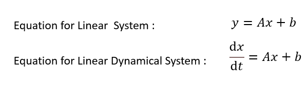
To know the usability of the Kalman Filter, we need to have a little bit of intuition about the Linear Dynamical System. A dynamical system evolves throughout time, so it’s a function of time. Most of the systems that we see in real life are dynamical systems. We have a particular branch of mathematics known as Calculus which describes a dynamic system very well. It works in the area where we deal with change rates overtime or any other parameters.

We call it a differential equation, right? So, if a set of differential equations describes a system, we call it a Linear Dynamic System. We must develop an algorithm to check an autonomous car’s position (latitude and longitude), direction, velocity, and other parameters. Now the position is nothing but a distance. And distance and velocity can be described with the help of differential equations, like rate of change in position or rate of change in direction or rate of change in velocity, etc.

Kalman Filter and Hidden Markov Model

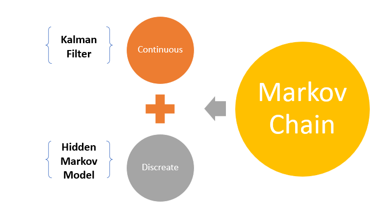
The Kalman Filter is a method for solving the continuous version of Hidden Markov Models. Hidden Markov deals with latent variables. Let me give a little bit of intuition. When you see a happy face in a crowd, you don’t know the reason for their happiness. There can be many factors like the guy got a job, or meet someone, etc. these factors are latent or hidden because you see only the outcome(happiness).

Markov chain says that only your present determines your future, not the past. For our happiness example with Hidden Markov Model, we want to determine the factors or variables(hidden) that cause feelings of happiness before the happy expression(outcome). I have written an article about Markov chain you can check that for more. Below I have given the link for the same.

In Hidden Markov Model, we assume the hidden state is one of a few classes, and the movement among these states uses a discrete Markov Chain. Whereas, in Kalman filters, we consider that the unobserved state distribution is Gaussian and moves continuously according to linear dynamics. So obviously, the precision will increase. In case we try to measure a value.

Measurement System Analysis and Kalman Filter

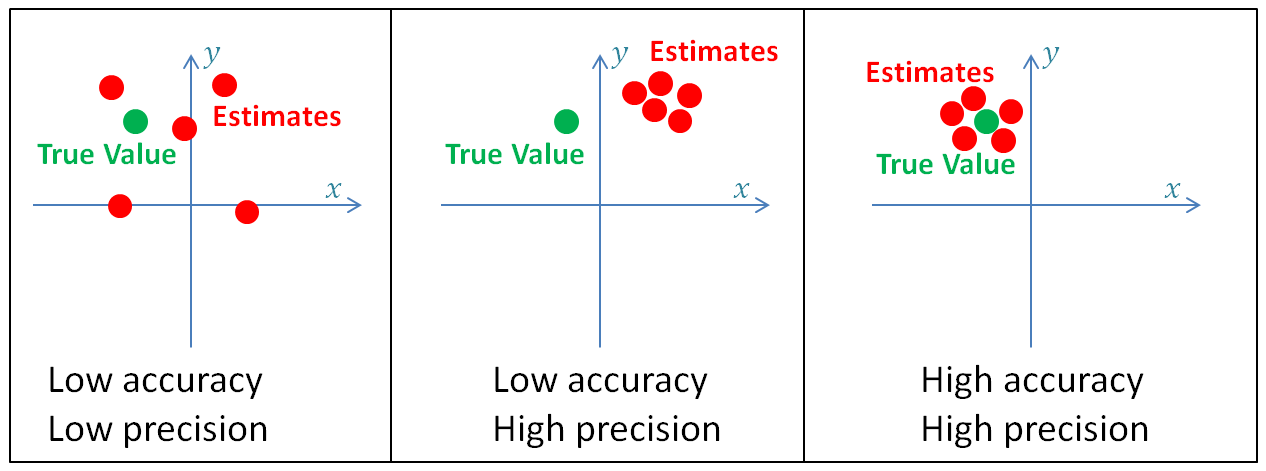
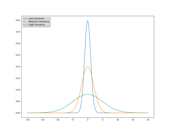
The core objective of a machine learning model is to predict or estimate a value or class, which will be closure to an accurate value or class. When we evaluate the hidden state of the system, we call it estimation. Like inbuilt accelerometer sensor in our smartwatch estimate our step counts or velocity. GPS sensor can calculate our position during the walk. This estimation has to be accurate means close to the actual value. Also, it needs to be precise, which speaks about the variability in measurement. Higher precision means lower variance meaning low uncertainty, while lower precision systems have higher variance meaning high uncertainty. The random measurement error produces the variance. By averaging or smoothing measurements, we can remove the variance. To get a closer estimation, we need more measurements data. Mainly continuous hidden data. Kalman filter advocates about it.

Why use Kalman filters?

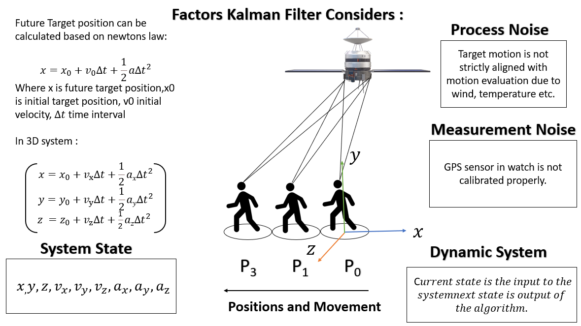
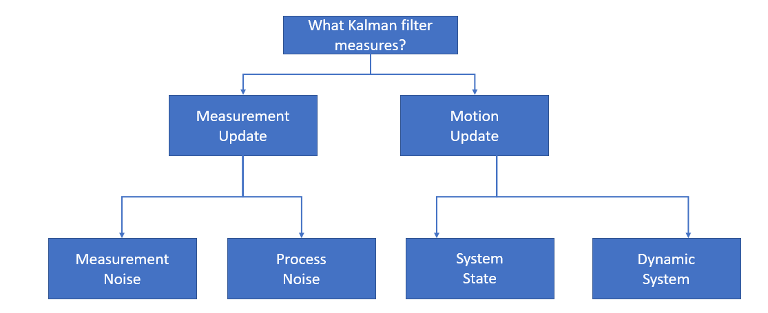
Let’s consider our first example. Our smartwatches have GPS sensors to track our physical movement during walking or running based on position or location coordinates. The most challenging part is giving you accurate and precise data—many external hidden factors like thermal noise, receiver clock precession, materials, GPS satellite location, etc., create problems in accuracy and precession. The Kalman filter estimates these hidden variables based on inaccurate and uncertain measurement, as it also provides a future state prediction based on the previous estimation. The below image gives some intuition of the factors that the Kalman filter considers.

Take another example of an Autonomous car. In an autonomous vehicle, inbuilt sensors determine the position of objects surrounding the vehicle. Also, a model that predicts the future positions of the objects. The issue with it in real-time system predictive model and sensors may not work well it leads to uncertainty. But with The Kalman filter, we can curb the uncertainty impact with the help of a distribution. More often, a gaussian distribution.

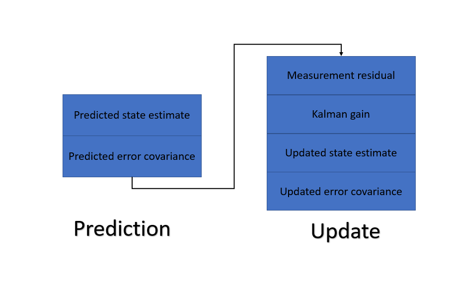
The internal process of a Kalman Filter

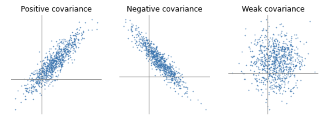
Kalman filter has two stages. It is a recursive process based on the continuous Markov chain. The two steps of it are two predicts and update. “prediction” and “update” are called “propagation” and “correlation.” Before we describe the process, lets us express one statistical term,’ Covariance.’ When we try to find the relation between two variables, we use two words Covariance and correlation. In the case of Covariance, we try to determine how much movement in one variable predicts the movement in corresponding variables. Covariance focuses on direction, not on strength. You can get some intuitive ideas from the below images about variance.

The Kalman Filter process model defines the evolution of the state from time t−1 to time t as:

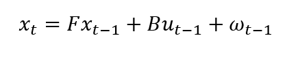
Here F is the state transition matrix that has been applied to the previous state vector x_t−1 , B is the control-input matrix used to the control vector u_t−1 , and w_t−1 is the process noise vector considered zero-mean Gaussian with the covariance Q.

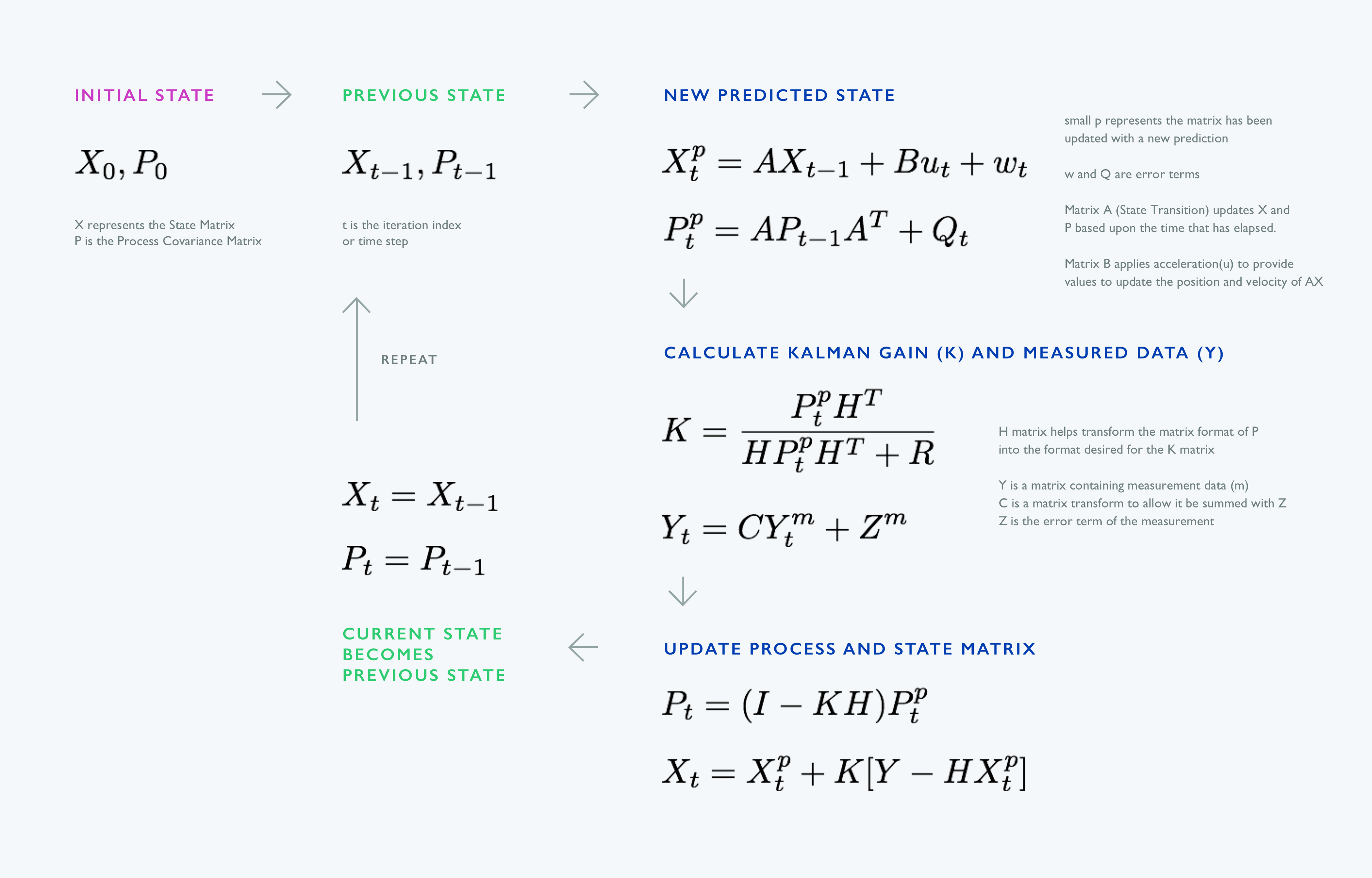
I won’t confuse you with the equations since the article is an intuitive picture of the Kalman filter. But one more important term I need to define without any equation. Calculating the Kalman gain(K) involved calculating the covariance matrix for the observation errors and comparing it with the process covariance matrix. In the case of Kalman Gain(K)–> 1, the measurements are accurate, but the estimates are unstable. A smaller value of Kalman gain means estimates are more stable, and the measurements are inaccurate.

Where to use The Kalman filter

It is an exciting question that where the Kalman filter Python can be used. Everywhere. Any data capturing process can use the Kalman filter. Like Sensors, as we are not sure if the sensor’s measurement data is right or wrong. Data capturing during speech and image processing. Most of the uses case can be found in Space related activities.

Code:

#Install(in Windows) :
pip install filterpy

#Considering a filter that tracks position and velocity using a sensor. only reads position:
from filterpy.kalman import KalmanFilter
f = KalmanFilter (dim_x=2, dim_y=1)

#Assign some initial value for the state (position and velocity):
f.x = np.array([[2.],    # position
                [0.]])   # velocity

#Define the state transition matrix:
f.F = np.array([[1.,1.],
                [0.,1.]])

#Define the measurement function:
f.H = np.array([[1.,0.]])

#Define the covariance matrix.
f.P = np.array([[1000.,    0.],
                [   0., 1000.] ])

#Assign the measurement noise. 
f.R = np.array([[5.]])

#Assign the process noise. 
from filterpy.common import Q_discrete_white_noise
f.Q = Q_discrete_white_noise(dim=2, dt=0.1, var=0.13)

#perform the predict/update loop:
z = get_sensor_reading()
f.predict()
f.update(z)
do_something_with_estimate (f.x)

Conclusion

In conclusion, Kalman Filter, a powerful tool in signal processing, excels in Linear Dynamical Systems, intertwines with Hidden Markov Models, and enhances Measurement System Analysis. Its versatility is showcased in various applications, offering a robust internal process. Explore coding examples to unleash the potential of Kalman filters across diverse domains.

Code Resource: https://filterpy.readthedocs.io/en/latest/kalman/KalmanFilter.html

Frequently Asked Questions

The media shown in this article is not owned by Analytics Vidhya and are used at the Author’s discretion.

Subhasis Sanyal 31 Jan 2024