This article was published as a part of the Data Science Blogathon.
Introduction
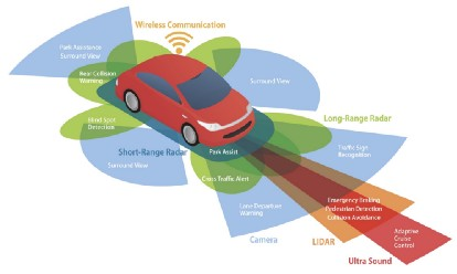
This article is an introduction to autonomous navigation. First, we will go through the basic concepts of LIDAR and see how sensor fusion helps to minimize the biases during measurement of the surrounding environment of the autonomous robot.
LIDAR stands for Light Detection and Ranging
LIDAR emits light waves into the surrounding environment, and these pulses bounce back and return to the sensor. Then the sensor measures the time to return and calculates the distance it traveled. Repeating this process creates a 3D environment map that can be used for the safe navigation of the robot.
Types of LIDAR sensor output
[1] LaserScan messages
[2] Point Cloud messages
Any LIDAR sensor can scan the area in front of it with a vision range. We define this vision range as angle_min and angle_max. We also consider angle increment at which particular angle the sensor takes the sample measurements. We also need to provide the time_increment which helps to take the samples at every time interval we define. For LIDAR, we have to detect if there is an obstacle in front of it or not. For this, we consider range_min and range_max. Here the range is an array. This array size depends on angle_increment and it stores the values of the maximum distance of the obstacle at that degree. If no obstacle is present, we take that element of the array as infinity (meaning no obstacle). If there is an obstacle, we assign that distance to it.
Using LIDAR, we can detect the objects and their exact object positions.
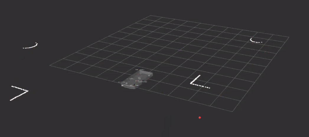
A laser scan was taken using a gazebo.
Dead reckoning is calculating the current position of the robot using the previous positions (as with Inertial Measurement Unit – IMU Sensor). But this process is highly susceptible to errors. Thus we use the concept of sensor fusion for localization.
Sensor Fusion
We are considering measurements from the combination of multiple sensors so that one sensor can compensate for the drawbacks of the other sensors. This is known as sensor fusion. We implemented sensor fusion using filters.
Types of filters:
[1] Kalman Filter [2] Complementary Filter [3] Particle FilterKalman Filter
Let us consider two sensors measuring distances from the sensor to the obstacles. Of which sensor 1 can measure short distances with high accuracy and sensor 2 can measure long distances with high accuracy. We want our robot to measure all the distances properly. So which sensor we consider for our measurements for the robot?
We take n measurements from these sensors and estimate the statistical properties of the measurement using PDF (probability density function).
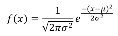
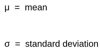
Here we can see that the probability density function is characterized by mean and standard deviation.
Here we take the n measurements from sensor 1 and sensor 2 and find the mean and standard deviation of these sensors. Then we find the probability density function for both the sensors.
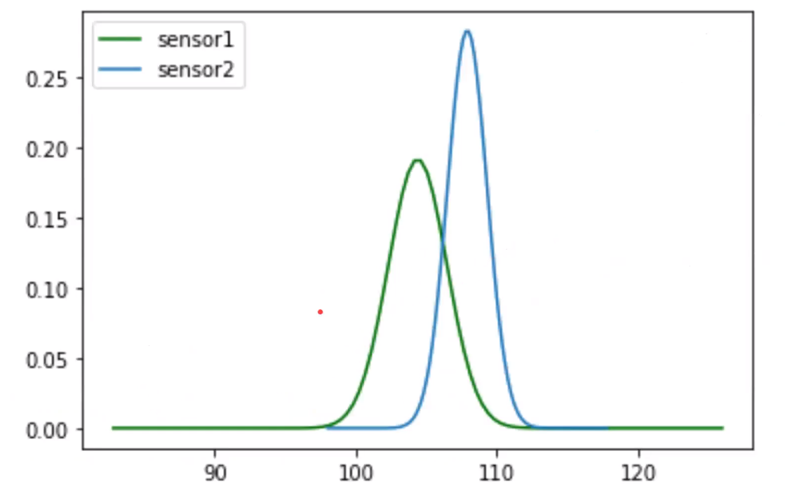
Probability Density Functions of sensor 1 and sensor 2.
Then how do we consider the true value of distance? Will you consider sensor 1 readings or sensor 2 readings? Here is where we use the Kalman filter.
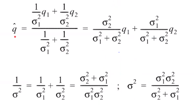
Here we find the new mean and standard deviation using the formulas below using the Kalman filter.
From the figure, we can say that we are more confident of our measurements from the new mean and new standard deviation.
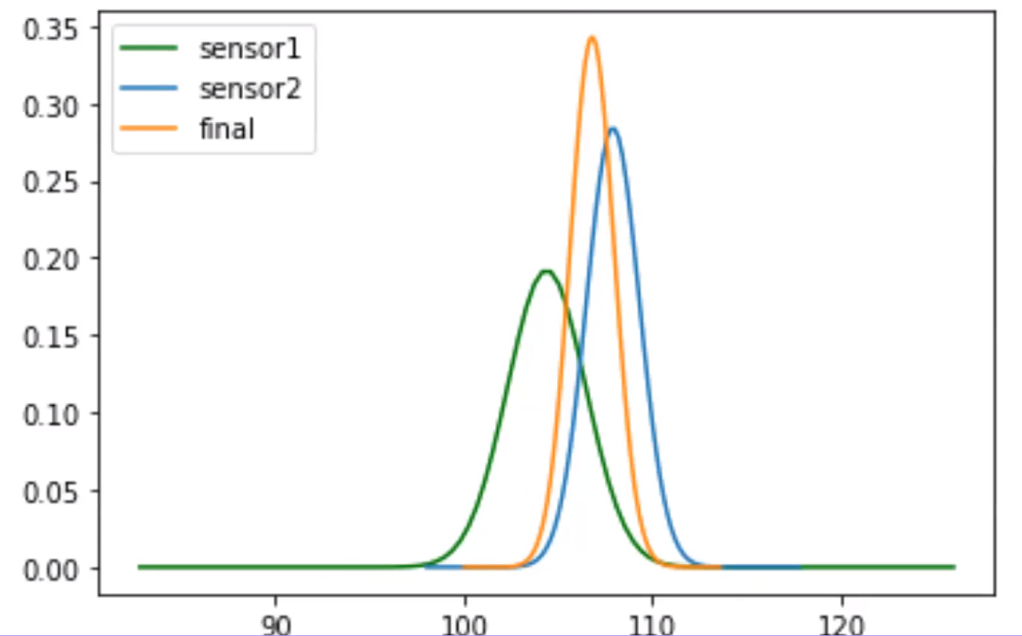
We can see that the new reading is narrower, which shows that we are more confident about our final readings with the new mean and standard deviation. This is an example of a static estimation case.
Example of dynamic estimation case
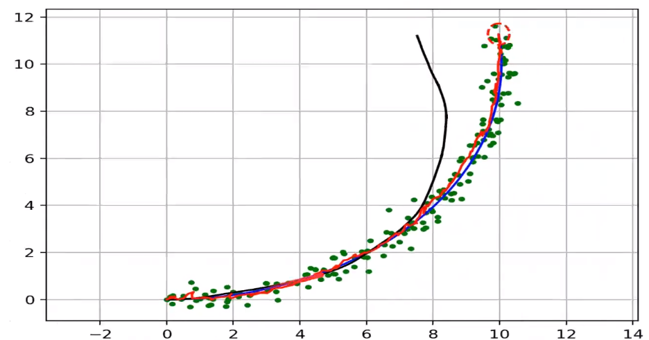
Blue line–Actual path of the robot
Black line–Position measurements using IMU (We can see that the error using IMU sensor by comparing the measurements from the blue path)
Green dots–Measurements from GPS
Red line–Sensor fusion using Kalman filter measurements considering measurements from IMU and GPS.
From the figure, we can see that we measure the actual path using sensor fusion on fusing sensors. From this, we can say that we are more confident about our final measurements by using the concept of Kalman filters.
Code for Kalman Filter in Python
import numpy as np
import matplotlib.pyplot as plt
import math
sensor_data1 = 100*np.ones(20)+8*np.random.rand(20)
sensor_data2 = 105*np.ones(20)+5*np.random.rand(20)
print('Sensor1_data :' , sensor_data1)
print('Sensor2_data :' , sensor_data2)
def find_meanvariance(sensor_data):
    mean = np.mean(sensor_data)
    variance = np.var(sensor_data)
    return [mean,variance]
m1,v1 = find_meanvariance(sensor_data1)
m2,v2 = find_meanvariance(sensor_data2)
print('mean1 = ', m1)
print('variance1 = ', v1)
print('mean2 = ', m2)
print('variance2 = ', v2)
def gaussian_dist(x,mean,variance):
    y = (1/np.power(2*np.pi*variance,0.5))*np.exp(-np.power(x - mean, 2.) / (2 * variance))
    return y
x1 = np.linspace(m1 - 5*v1, m1 + 5*v1, 100)
x2 = np.linspace(m2 - 5*v2, m2 + 5*v2, 100)
y1 = gaussian_dist(x1,m1,v1)
y2 = gaussian_dist(x2,m2,v2)
plt.plot(x1,y1,'g-',label='sensor1')
plt.plot(x2,y2,label='sensor2')
plt.legend(loc='upper left')
plt.show()
def m_v_new(m1,m2,v1,v2):
    #insert code here
    m_new=(m1*v2+m2*v1)/(v1+v2)
    v_new=(v1*v2)/(v1+v2)
    return [m_new,v_new]
# Plot the new gaussian distribution
m_new,v_new = m_v_new(m1,m2,v1,v2)
x_new = np.linspace(m_new - 5*v_new, m_new + 5*v_new, 100)
y_new = gaussian_dist(x_new,m_new,v_new)
plt.plot(x1,y1,'g-',label='sensor1')
plt.plot(x2,y2,label='sensor2')
plt.plot(x_new,y_new,label='final')
plt.legend(loc='upper left')
plt.show()
References
[1]https://taylor.raack.info/2017/09/autonomous-vehicle-technology-sensor-fusion-and-extended-kalman-filters-for-object-tracking/ [2]https://www.ness.com/sensor-fusion-algorithms-for-autonomous-driving-part-1%E2%80%8A- %E2%80%8Athe-kalman-filter-and-extended-kalman-filter/ [3]https://medium.com/lansaar/what-is-sensor-fusion-cb596f7cf446 [4]https://towardsdatascience.com/kalman-filter-an-algorithm-for-making-sense-from-the-insights-of-various-sensors-fused-together-ddf67597f35eThe media shown in this article on autonomous navigation are not owned by Analytics Vidhya and is used at the Author’s discretion.


