Credit Card Lead Prediction – Complete project using LGBM Classification model

This article was published as a part of the Data Science Blogathon

The objective of this article is to help you get started with how to complete an end-to-end project assuming that you are a beginner. As this article covers step by step guide so maybe it will be lengthy.

In this article, we will be dealing with a classification problem, and you will see how easy and simple it is. For this, we will use the Credit Card Lead Prediction Dataset. It is a dataset given on Analytics Vidhya – Jobathon event. You can easily download the dataset from here: Credit Card Lead Prediction Dataset.

Photo by Anna Shvets from Pexels

You can use any choice of notebooks like Jupyter, Google Colab, Kaggle, etc. to run the code.

Let’s get started,

About Dataset

• There is a Bank named Happy customer Bank which is a mid-sized private bank that deals in all kinds of banking products, like Savings accounts, Current accounts, investment products, credit products, among other offerings.
• The bank also cross-sells products to its existing customers and to do so they use different kinds of communication like tele-calling, e-mails, recommendations on net banking, mobile banking, etc.
• In this case, Happy Customer Bank wants to cross-sell its credit cards to its existing customers. The bank has identified a set of customers that are eligible for taking these credit cards.
• Bank wants to identify customers that could show higher intent towards a recommended credit card, given:

1. Customer details (gender, age, region, etc.)
2. Details of his/her relationship with the bank (Channel_Code, Vintage, Avg_Asset_Value, etc.)

Here, we have the task of building a model that’s capable of identifying customers who are interested in a credit card.

Importing Libraries

Importing necessary libraries such as NumPy for linear algebra, pandas for data processing, seaborn, and matplotlib for data visualizations.

import numpy as np 
import pandas as pd 
import matplotlib.pyplot as plt
import seaborn as sns

Loading Dataset

You can get the dataset from the above-given link.

df_train=pd.read_csv("train_s3TEQDk.csv")
df_train["source"]="train"
df_test=pd.read_csv("test_mSzZ8RL.csv")
df_test["source"]="test"
df=pd.concat([df_train,df_test],ignore_index=True)

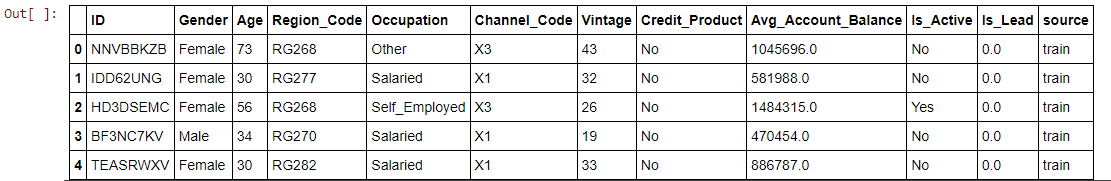
df.head()

Checking and Cleaning of Dataset

After loading the dataset the very next step is checking information about the dataset and cleaning the dataset which includes checking the shape, datatypes, unique values, null values.

#Checking shape 
df.shape

Observation: In our dataset, we have 351037 rows with 12 features after concatenating the train and test file.

#Check for Null Values
df.isnull().sum()

Observation: Null values are present in the Credit_Product feature.

Now we use the fillna method for filling null values in our dataset.

#Filling Null Values
df['Credit_Product']= df['Credit_Product'].fillna("NA")

Observation: We remove all the null values present in our dataset.

Moving forward, we have to check the data types of the features.

Observation: 

• Some categorical features need to be changed in numerical datatype.
• Here, we found that the Is_Active feature has two values i.e. Yes and No. So, we have to convert these values into float datatype.

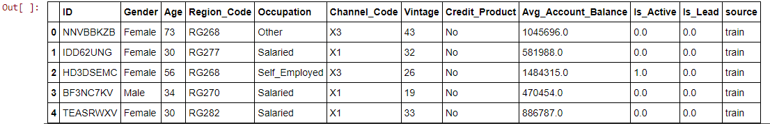
#Changing Yes to 1 and No to 0 in Is_Active column to covert  data into float
df["Is_Active"].replace(["Yes","No"],[1,0],inplace=True)
df['Is_Active'] = df['Is_Active'].astype(float)

df.head()

Now, for changing all categorical columns into numerical form here we use label encoding. Not to dive directly into applying label encoding, let’s understand briefly what exactly label encoding is.

Label Encoding: Label Encoding refers to converting the labels into the numeric form for converting it into the machine-readable form. It is a popular encoding technique for handling categorical variables.

Using Label Encoder:

#Creating list of categorical columns
cat_col=[ 'Gender', 'Region_Code', 'Occupation','Channel_Code', 'Credit_Product']
from sklearn.preprocessing import LabelEncoder
le = LabelEncoder()       #creating instance
for col in cat_col:
  df[col]= le.fit_transform(df[col])
df_2= df
df_2.head()

At this point, we can drop features that are irrelevant and have no effect on our dataset. Here we have two columns to drop i.e. ‘ID’ and ‘source’. Let’s check the latest output. 

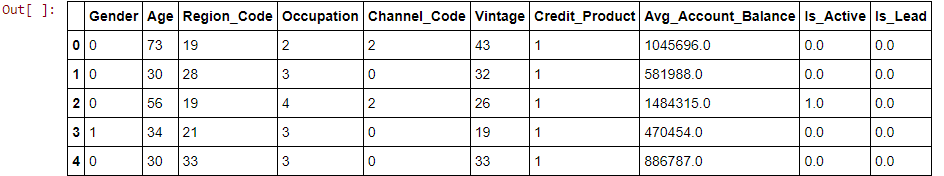
Now, we observed that all the data are in numerical form.

Moving to our next step is data visualizations.

Data Visualization

For gathering insights, data visualization is a must.

a. Univariate Analysis: First, we plotted the dist plot and count plots to understand the distribution of data.

•  The dist plot for the ‘Age’ feature:

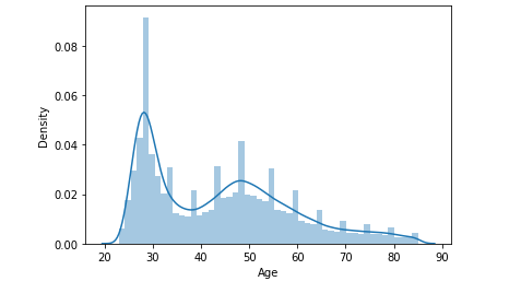
Observation: 

1. The Age distribution is slightly skewed towards the left i.e. “Positive Skew”.
2. In this, we see that one age group is younger between 20 to 40 years of age while the other is 40 to 60 years of age. In addition to this, those in the range of 40 to 60 have leads whereas younger ones aren’t.
3. So, this could be associated with the ‘Vintage’ variable which would be more visible for the higher age group.

• The count plot for the ‘Gender‘ feature:

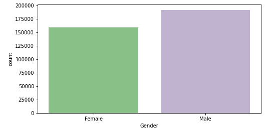
Observation: 

1. There are more male customers present in the dataset. But the gender of the customer does not really matter in deciding who has a better lead.

• The count plot for the ‘Is_Lead‘ feature (target variable):

 

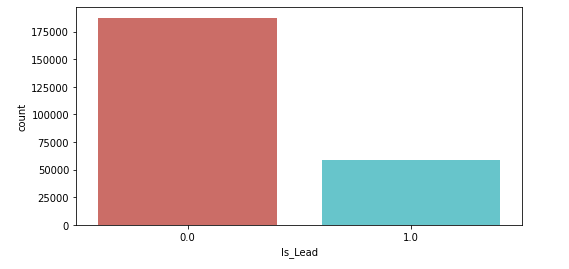
Observation: 

1. The plot shows that the data is highly imbalanced and needs to be corrected or balanced before applying different algorithms.
2. To balance the dataset we use undersampling techniques in further steps.

b. Bivariate Analysis:  Now, we do some bivariate analysis for understanding the relationship between different columns.

• ‘Occupation’ with ‘Customers’:

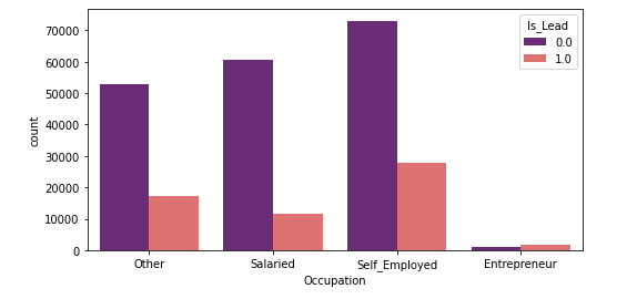
Observation:  

1. We observe that self-employed customers are less likely to get a credit card. Whereas, entrepreneurs (though limited) are most likely to get a credit card.

•  The ‘Activeness of customers’ in last 3 months to ‘Occupation of customers’:

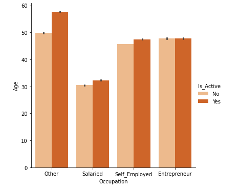
Observation:

1. Here, we observed that the active customers are more in a salaried, self-employed, and others as compared to the entrepreneur in last 3 months.
2. There are quite a lot of customers who are not active in the last 3 months compared to those who are active.
3. The proportion of leads for ‘Active‘ customers is higher as compared to ‘Non-active‘ customers.

Now, our data visualization part is over.

Data Preparation for Credit Card Lead Prediction

As we see previously that our targeted variable is imbalanced and needed to be corrected for proper modeling.

So to balance the dataset we will apply the undersampling method.

For this, firstly, we will import a library. Then separate the minority and majority classes.

from sklearn.utils import resample
# separate the minority and majority classes
df_majority = df_1[df_1['Is_Lead']==0]
df_minority = df_1[df_1['Is_Lead']==1]

print(" The majority class values are", len(df_majority))
print(" The minority class values are", len(df_minority))
print(" The ratio of both classes are", len(df_majority)/len(df_minority))

Observation:  We got the majority class values are 126800, minority class values 63400, and the ratio of both classes is 2.0.

Now, we have to combine the minority class with the oversampled majority class.

# undersample majority class
df_majority_undersampled = resample(df_majority, replace=True, n_samples=len(df_minority), random_state=0)
# combining minority class with oversampled majority class
df_undersampled = pd.concat([df_minority, df_majority_undersampled])

df_undersampled['Is_Lead'].value_counts()
df_1=df_undersampled

After this, we have to calculate new class value counts.

# display new class value counts
print(" The undersamples class values count is:", len(df_undersampled))
print(" The ratio of both classes are", len(df_undersampled[df_undersampled["Is_Lead"]==0])/len(df_undersampled[df_undersampled["Is_Lead"]==1]))

Observation:  

• The undersample class values count is 126800.
•  The ratio of both classes is 1.0.

It’s time to drop our target variable and assigning the value of y for the training and testing phase.

# dropping target variable 
xc = df_1.drop(columns=['Is_Lead'])
yc = df_1[["Is_Lead"]]

Now, here I used Standard Scaler for standardizing the value of x to make the data normally distributed.

sc = StandardScaler()        #instance of Standard Scaler
df_xc = pd.DataFrame(sc.fit_transform(xc),columns=xc.columns)

Finally, we are ready with our data for the modeling task.

 Classification Modeling

Let’s start with importing the necessary libraries for classification modeling. 

Now we checked various classification models and calculated metrics such as precision, recall, ROC_AUC score, and F1 score.

 Here, the models used are:-

1. Logistic Regression
2. Random Forest Classifier
3. Decision Tree Classifier
4. Gaussian NB Classifier

Observation:

 

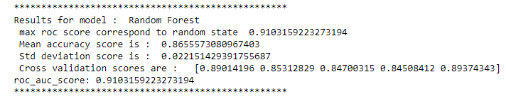
From all the initial model performances, we see that Random Forest Classifier performs better than others having maximum accuracy-score and minimum standard deviations.

Now, to increase our accuracy even further, we will perform Hyperparameter tuning.

For hyperparameter tuning, we have to find the best parameter i.e. ‘n_estimators’ using GridSearchCV for our model.

# Estimating best n_estimator using grid search for Randomforest Classifier
parameters={"n_estimators":[1,10,100]}
rf_clf=RandomForestClassifier()
clf = GridSearchCV(rf_clf, parameters, cv=5,scoring="roc_auc")
clf.fit(df_xc,yc)
print("Best parameter : ",clf.best_params_)

Observation:

 

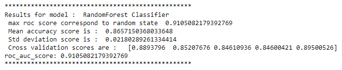
Again running Random Forest Classifier with best parameter i.e. ‘n_estimators’ = 100.

rf_clf=RandomForestClassifier(n_estimators=100,random_state=42)
max_accuracy_scr("RandomForest Classifier",rf_clf,df_xc,yc)

Observation:

 

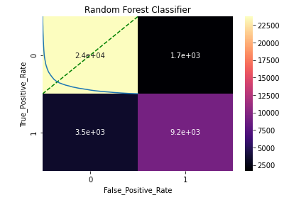
Now, to check model performance we will plot different performance metrics such as confusion matrix, classification report, and AUC_ROC curve.

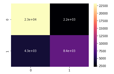
a. Confusion Matrix:  A confusion matrix is a performance measurement technique for a classification model. It is a kind of table which helps to know the classification model on a set of test data for that the true values are known.

#Plotting confusion matrix
cnf = confusion_matrix(yc_test,yc_pred)
sns.heatmap(cnf, annot=True, cmap = "magma")

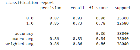
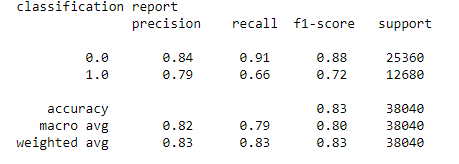
b. Classification Report:  A classification report is a performance evaluation metrics. It is used to show the precision, recall, F1 score, and support of the trained classification model.

c. AUC_ROC Curve: AUC_ROC curve is a performance measurement for classification problems at various thresholds settings. ROC is a probability curve and AUC represents the degree or measure of separability. It tells how much the model is capable of distinguishing between classes.

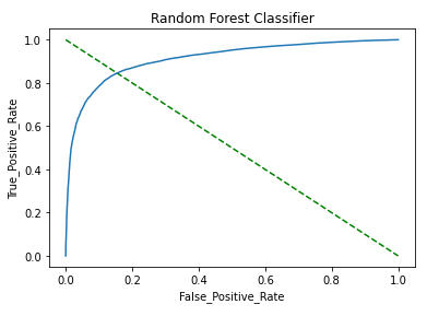
Observation: 

• Found a decent accuracy score (~0.86), precision, and recall for the model.
• The AUC_ROC curve shows a good match between the test and predicted values.
• Overall this indicates that the model is a good fit for the prediction.

Now, here to boost the accuracy and ROC_AUC score I attempted to use XG Boost Classifier as it is inherently well suited for the imbalanced classification problems.

As this article goes lengthy so here, I will be showing only outputs and not code snippets. So if you want you can check the complete code from the link given at the end of this article.

Now, coming to our XG Boost results we have got a good ROC_AUC score (~0.87). To check model performance we will plot different performance metrics.

a. Confusion Matrix:

b. Classification Report:

c. AUC_ROC Curve:

 

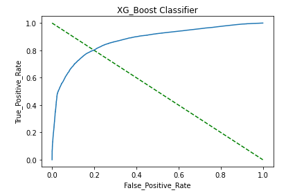
Observation:

• Plotted AUC_ROC Curve that shows a good match between the test and predicted values.
• Found max ROC score is 0.87.
• Overall model fit is good.
• However, the XG Boost AUC score with test data dropped to ~0.86 due to overfitting issues.

So, to avoid the issue of overfitting in the dataset I decided to implement stratification folds and also use the LGBM model for finding classification-based probabilities.

Stratified K-Folds cross-validator – It provides train/test indices to split data into train/test sets. This cross-validation object is a variation of K-Fold that returns stratified folds. The folds are made by preserving the percentage of samples for each class.

Here, I used 10 stratified cross-folds with different parameters.

#Applying LGBM Model with 10 stratified cross-folds
from lightgbm import LGBMClassifier

lgb_params= {'learning_rate': 0.045, 'n_estimators': 10000,'max_bin': 84,'num_leaves': 10,'max_depth': 20,'reg_alpha': 8.457,'reg_lambda': 6.853,'subsample': 0.749}
lgb_model = cross_val(xc, yc, LGBMClassifier, lgb_params)

After running the LGBM algorithm, we found a good ROC_AUC score (~0.87). Now it’s time to check model performance with different metrics.

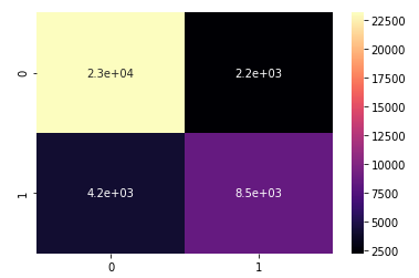
 a. Confusion Matrix:

 

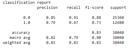
b. Classification Report:

c. AUC_ROC Curve:

 

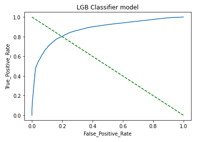
Observation:

• The model performed very well with the test data and provided an AUC score of ~0.871.
• This was done to remove any overfitting issues in the model.
• Plotted performance metrics i.e. AUC_ROC curve that shows a good match between test and predicted values.

Prediction of Credit Card Lead

Preparing dataset for prediction.

1. We can drop column which is irrelevant and has no effect on our data such as ‘source’ column.

df_3 = df_test

df_3.drop(columns=["source"],inplace=True)

df_3.head()

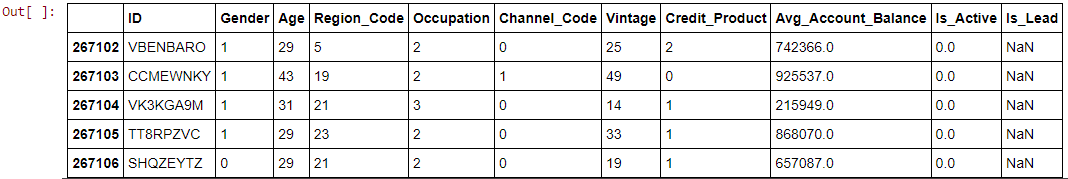
2. Now dropping the target variable from the test dataset.

xc_pred = df_3.drop(columns=['Is_Lead',"ID"])

3. Standardizing the value of x by using a standard scaler to make the data normally distributed.

sc = StandardScaler()
df_xc_pred = pd.DataFrame(sc.fit_transform(xc_pred),columns=xc_pred.columns)

lead_pred_xg=clf2.predict_proba(df_xc_pred)[:,1]
lead_pred_lgb=lgb_model.predict_proba(df_xc_pred)[:,1]
lead_pred_rf=rf_clf.predict_proba(df_xc_pred)[:,1]
print(lead_pred_xg, lead_pred_lgb, lead_pred_rf)

4. Creating data frames for Lead Prediction.

#Dataframe for lead prediction
lead_pred_lgb= pd.DataFrame(lead_pred_lgb,columns=["Is_Lead"])
lead_pred_xg= pd.DataFrame(lead_pred_xg,columns=["Is_Lead"])
lead_pred_rf= pd.DataFrame(lead_pred_rf,columns=["Is_Lead"])

5. Saving ‘ID’ and prediction to the csv file for all the models.

#Saving ID  and prediction to csv file for LGB Model
df_pred_lgb=pd.concat([df_test["ID"],lead_pred_lgb],axis=1,ignore_index=True)
df_pred_lgb.columns = ["ID","Is_Lead"]
print(df_pred_lgb.head())
df_pred_lgb.to_csv("Credit_Card_Lead_Predictions_final_lgb.csv",index=False)

Similarly, we did it for Random Forest and XGBoost model.

Output:  LGBM model

 

Hence, LGBM is selected as a final model as it is the most consistent model with the highest AUC score.

Saving the Credit Card Lead Prediction model

First, import the library and save the model as a pickle in a file.

import joblib

joblib.dump(lgb_model,'lgb_model.pkl')

End Notes

This ends our project. ‘Cheers!!!’

For a complete project check out my solution and dataset from the below link:

https://github.com/priyalagarwal27/Credit-Card-Lead-Prediction

Please leave any suggestions, questions for further clarification. Hope this would be helpful for you and you liked it as well. HAPPY READING!!!!

About the Author:

Priyal Agarwal 

Connect me on LinkedIn or mail me at [email protected].

Priyal Agarwal 06 Oct 2021

My name is Priyal Agarwal. Recently I've completed a PG program in data science, Machine Learning, and neural networks and I've experienced as a data science intern in Fliprobo technologies, Bangalore as well. I am an enthusiastic, self-motivated, reliable, dedicated and open- minded person. I get across to people and adjust to changes with ease. I believe that a person should work on developing their professional skills and learning new things all the time. For that, I write technical blogs/articles on medium and Analytics Vidhya in contribution to the Data Science Community and learn about new technologies to excel my knowledge.