Overview
Data provides us with the power to analyze and forecast the events of the future. With each day, more and more companies are adopting data science techniques like predictive forecasting, clustering, and so on. While it’s very intriguing to keep learning about complex ML and DL algorithms, one should not forget to master the essential data preprocessing. One of the important parts of data pre-processing is handling missing values. This is a complete guide on how to deal with different types of missing data.
This article was published as a part of the Data Science Blogathon
Table of contents
- Why is it important to handle missing data?
- Reasons behind Missing Values
- Types of Missing Values
- Check for missing values
- Visualizing missing values with Missingno
- Dropping rows with missing values
- Imputation for continous variable
- Predicting the missing values with Regression
- Missing values in categorical data
- How to handle missing values in Time series data?
- Conclusion
Why is it important to handle missing data?
The data in the real world has many missing data in most cases. There might be different reasons why each value is missing. There might be loss or corruption of data, or there might be specific reasons also. The missing data will decrease the predictive power of your model. If you apply algorithms with missing data, then there will be bias in the estimation of parameters. You cannot be confident about your results if you don’t handle missing data.
Reasons behind Missing Values
Ever wondered about the reasons behind missing data in datasets?
Some of the possible reasons behind missing data are:
- People do not give information regarding certain questions in a data collection survey. For example, some may not be comfortable sharing information about their salary, drinking, and smoking habits. These are left out intentionally by the population
- In some cases, data is accumulated from various past records available and not directly. In this case, data corruption is a major issue. Due to low maintenance, some parts of data are corrupted giving rise to missing data
- Inaccuracies during the data collection process also contribute to missing data. For example, in manual data entry, it is difficult to completely avoid human errors
- Equipment inconsistencies leading to faulty measurements, which in turn cannot be used.
Types of Missing Values
The missing data can occur due to diverse reasons. We can categorize them into three main groups: Missing Completely at Random, Missing At Random, Not Missing at Random.
1. Missing Completely at Random (MCAR)
The missing data do not follow any particular pattern, they are simply random. The missing of these data is unrelated or independent of the remaining variables. It is not possible to predict these values with the rest of the variable data. For example, during the collection of data, a particular sample gets lost due to carelessness. This is an ideal case, where statistically the analysis will not be biased. But you shouldn’t assume the presence of MCAR unless very sure as it is a rare situation.
2. Missing At Random (MAR)
Here unlike MCAR, the data is missing amongst particular subsets. It is possible to predict if the data will be present/absent with the help of other features. But, you cannot predict the missing data themselves.
For example, let us consider a survey about time spent on the internet, which has a section about time spent on platforms like Netflix, amazon prime. It is observed that older people( above 45 years) are less likely to fill it than younger people. This is an example of MAR. Here, the ‘Age’ parameter decides if the data will be missing or not. MAR occurs very commonly than MCAR.
3. Not Missing at Random (NMAR)
This is a serious and tricky situation. Let’s say the purpose of the survey is to measure the overuse/addiction to social media. If people who excessively use social media, do not fill the survey intentionally, then we have a case of NMAR. This will most probably lead to a bias in results. The usual methods like dropping rows/columns, imputation will not work. To solve this, in-depth knowledge of the domain would be necessary.
Now that we have seen the different types of missing data, let’s move ahead to the various ways of handling them.
Check for missing values
When you have a dataset, the first step is to check which columns have missing data and how many. Let us use the most famous dataset among Data science learns, of course, the Titanic survivor! Read the dataset using pandas read_csv function as shown below.
import pandas as pd
train=pd.read_csv('train.csv')
test=pd.read_csv('test.csv')
print('Training data shape: ', train.shape)
print('Testing data shape: ', test.shape)
print(train.head())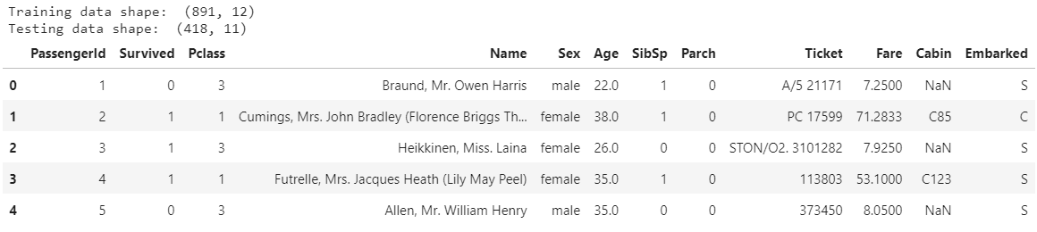
Source: Image from Author’s Kaggle notebook
Now we have the training and test data frames of titanic data.
How to check which columns have missing data, and how many?
The ” isnull()” function is used for this. When you call the sum function along with isnull, the total sum of missing data in each column is the output.
missing_values=train.isnull().sum()
print(missing_values)
PassengerId 0
Survived 0
Pclass 0
Name 0
Sex 0
Age 177
SibSp 0
Parch 0
Ticket 0
Fare 0
Cabin 687
Embarked 2
dtype: int64Notice that 3 columns have missing values: Age, Cabin, Embarked
Although we know how many values are missing in each column, it is essential to know the percentage of them against the total values. So, let us calculate that in a single line of code.
mis_value_percent = 100 * train.isnull().sum() / len(train)
print(mis_value_percent)
PassengerId 0.000000
Survived 0.000000
Pclass 0.000000
Name 0.000000
Sex 0.000000
Age 19.865320
SibSp 0.000000
Parch 0.000000
Ticket 0.000000
Fare 0.000000
Cabin 77.104377
Embarked 0.224467
dtype: float64It is clear that 77% of the ‘Cabin’ Column is missing, which is a very significant percentage. Age has around 19% of data missing and Embarked has only 0.2% missing. This is the quantitative analysis of missing data we have. What about qualitative? Keep reading!
Visualizing missing values with Missingno
Guess what? We have a python package especially for visualizing and exploring the missing data of a dataset. The “Missingno” python package. Go ahead and install it quickly
pip install missingnoUsing this, we can make visualizations in the form of heat maps, bar charts, and matrices. By analyzing how they are distributed, you can conclude what category they fall into MCAR, MAR, or NMAR. We can also find the correlation of the columns containing the missing with the target column
Start by making a bar chart for non-null values using the ‘bar()’ function of the missingno library. You have passed the pandas dataframe to this function.
import missingno as msno
msno.bar(train)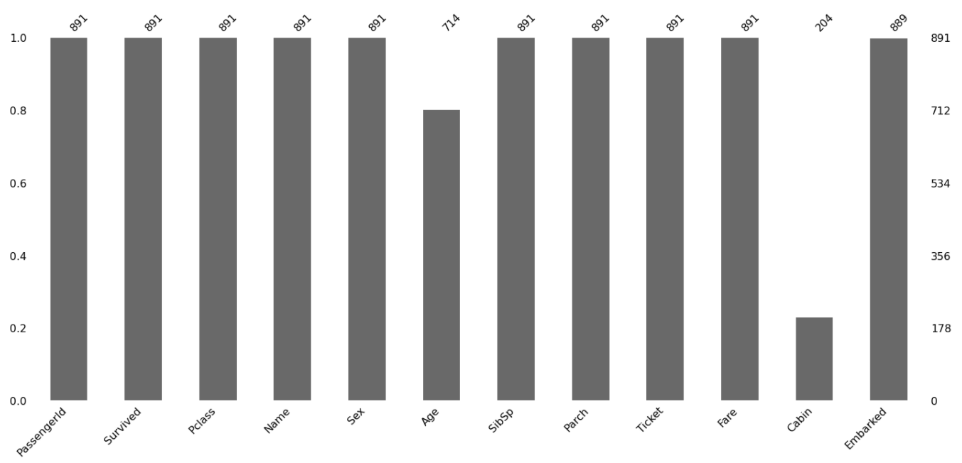
Source: Image from Author’s Kaggle notebook
Next, we can plot the matrix visualization. This helps us to know how the missing data is distributed through the data, that is if they are localized or evenly spread, or is there any pattern and many such questions.
msno.matrix(train)
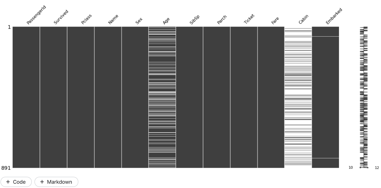
In the matrix plot, you will see blank lines for each missing data. Notice that the ‘Embarked’ column has just two random missing data, which follow no pattern. They were probably lost during data acquisition. So, this can be classified as Missing completely at Random.
The age and Cabin columns could possibly be MAR. But we want to ensure that there are no correlations between them.
How to do that?
Lucky for us, missingno package also provides the ‘heatmap’ function. Using this we can find if there are any correlations between missing data of different columns.
msno.heatmap(train)Output is shown!
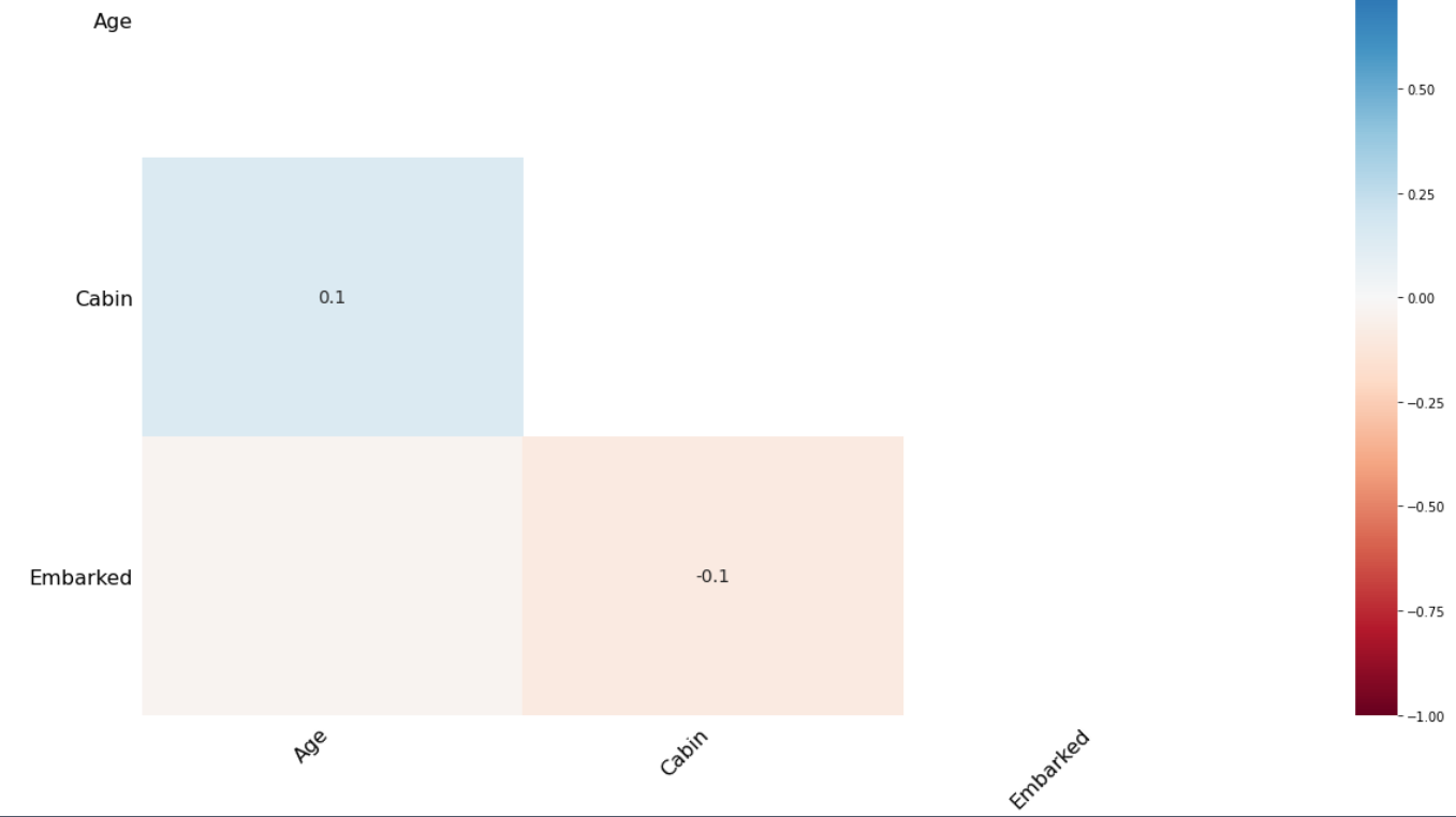
The heatmap shows there is no such strong correlation between the missing data of the Age and Cabin column. So, the missing data of these columns can be classified as MAR or Missing at Random.
I hope you are clear about how to analyze missing values. Next, I will move on to discussing the different ways of handling these missing data.
Dropping rows with missing values
It is a simple method, where we drop all the rows that have any missing values belonging to a particular column. As easy as this is, it comes with a huge disadvantage. You might end up losing a huge chunk of your data. This will reduce the size of your dataset and make your model predictions biased. You should use this only when the no of missing values is very less.
For example, the ‘Embarked’ column has just 2 missing values. So, we can drop rows where this column is missing. Follow the below code snippet.
print('Dataset before :', len(train))
train.dropna(subset=['Embarked'],how='any',inplace=True)
print('Dataset after :', len(train))
print('missing values :',train['Embarked'].isnull().sum())
Dataset before : 891
Dataset after : 889
missing values : 0Imagine if you did the same for the ‘Age’ column. You would lose like 77% of your data!
Dropping columns
When a column has large missing values, there is no point in imputing the values with the least available true data we have. So, when any column has greater than 80% of values missing, you can just drop that column from your analysis. In our case, ‘Cabin’ has 77% data missing, so you can take the choice of dropping this column.
Make sure that the dropped column is not crucial for your analysis. If so, you should try to get more data and then impute the missing values.
Imputation for continous variable
When you have numeric columns, you can fill the missing values using different statistical values like mean, median, or mode. You will not lose data, which is a big advantage of this case.
Imputation with mean
When a continuous variable column has missing values, you can calculate the mean of the non-null values and use it to fill the vacancies. In the titanic dataset we have been using until now, ‘Age’ is a numeric column. Look at the first few values of it and notice it has ‘NaN’ at row 5.
train['Age'][:10]0 22.0
1 38.0
2 26.0
3 35.0
4 35.0
5 NaN
6 54.0
7 2.0
8 27.0
9 14.0
Name: Age, dtype: float64Now, lets us perform mean imputation on this column
train['Age']=train['Age'].replace(np.NaN,train['Age'].mean())
train['Age'][:10]
0 22.000000
1 38.000000
2 26.000000
3 35.000000
4 35.000000
5 29.699118
6 54.000000
7 2.000000
8 27.000000
9 14.000000
Name: Age, dtype: float64You can see that the ‘NaN’ has been replaced with 29.699 (the computed mean).
Mean imputation has certain disadvantages. If the data has a very uneven distribution, with many outliers, then the Mean will not reflect the actual distribution of the data. Mean is affected greatly by extreme values or outliers. So, if the data doesn’t have many outliers and follows near-normal distribution, use mean imputation
Imputation with Median
The missing values of a continuous feature can be filled with the median of the remaining non-null values. The advantage of the median is, it is unaffected by the outliers, unlike the mean. Let us implement it here.
train['Age']=train['Age'].replace(np.NaN,train['Age'].median())
train['Age'][:10]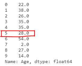
You can observe that the median value(28.0) has been filled inplace of NaN values.
Similarly, you can perform mode imputation also. Generally, Imputation with the mode is popular for categorical missing values. I’ll cover that in-depth in a later section
Predicting the missing values with Regression
Instead of filling a single mean or median value in all places, what if we can predict them with help of other variables we have?
Yes! We can use the features with non-null values to predict the missing values. A regression or classification model can be built for the prediction of missing values. Let us implement this for the ‘Age’ column of our titanic dataset.
We can process the data for building the model. The “Age” feature will be the target variable.
x_train: The rows of the dataset that have the “Age” value present are filtered. The ‘Age’ is target x_test: It is the “Age” column with non-null values
The y_train will have the data which have missing Age values, which shall be predicted (y_pred)
import pandas as pd
data=pd.read_csv('../input/titanic/train.csv')
data = data[["Survived", "Pclass", "Sex", "SibSp", "Parch", "Fare", "Age"]]
data["Sex"] = [1 if x=="male" else 0 for x in data["Sex"]]
test_data = data[data["Age"].isnull()]
data.dropna(inplace=True)
x_train = data.drop("Age", axis=1)
x_test = test_data.drop("Age", axis=1)
y_train = data["Age"]
Let us fit a Linear Regression Model to these data. I’ll be using the sklearn library here.
from sklearn.linear_model import LinearRegression
model = LinearRegression()
model.fit(X_train, y_train)
y_pred = model.predict(X_test)
Now, we have the null values of the Age column predicted in y_pred.
I will print out few examples of the test input and the predicted output for your better understanding.
print(x_test[:10])Survived Pclass Sex SibSp Parch Fare
5 0 3 1 0 0 8.4583
17 1 2 1 0 0 13.0000
19 1 3 0 0 0 7.2250
26 0 3 1 0 0 7.2250
28 1 3 0 0 0 7.8792
29 0 3 1 0 0 7.8958
31 1 1 0 1 0 146.5208
32 1 3 0 0 0 7.7500
36 1 3 1 0 0 7.2292
42 0 3 1 0 0 7.8958This is how inputs are passed to the regression model. Let’s look at the predicted age values.
print(y_pred[:10])[29.07080066 30.10833306 22.44685065 29.08927347 22.43705181 29.07922599
32.43692984 22.43898701 22.15615704 29.07922599]Hurray! We got the values.
Missing values in categorical data
Until now, we saw how to deal with missing numerical data. What if data is missing in the case of a categorical feature? For example, the “Cabin” feature of the Titanic dataset is categorical. Here, we cannot compute mean and median. So, we can fill the missing values with the mode or most frequently occurring class/category.
train['Cabin']=train['Cabin'].fillna(train['Cabin'].value_counts().index[0])When the percentage of missing values is less, this method is preferred. It does not cause a huge loss of data, and it is statistically relevant.
But if you have a lot of missing values, then it doesn’t make sense to impute with the most frequent class. Instead, let us create a separate category for missing values like “Unknown” or “Unavailable”. The number of classes will be increased by one.
When missing values is from categorical columns (string or numerical) then the missing values can be replaced with the most frequent category. If the number of missing values is very large then it can be replaced with a new category.
train['Cabin']=train['Cabin'].fillna('Unknown')
train['Cabin'][:10]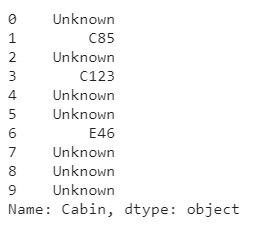
It works well with a small dataset. It also negates the loss of data by adding a unique category.
How to handle missing values in Time series data?
The datasets where information is collected along with timestamps in an orderly fashion are denoted as time-series data. If you have missing values in time series data, you can obviously try any of the above-discussed methods. But there are a few specific methods also which can be used here.
To get an idea, I’ll create a simple dummy dataset.
time= pd.date_range("1/01/2021", periods=10, freq="W")
df = pd.DataFrame(index=time);
df["Units sold"] = [5.0,4.0,np.nan,np.nan,1.0,np.nan,3.0,6.0,np.nan,2.0];
print(df)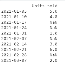
Let’s move on to the methods
Forward-fill missing values
The value of the next row will be used to fill the missing value.’ffill’ stands for ‘forward fill’. It is very easy to implement. You just have to pass the “method” parameter as “ffill” in the fillna() function.
forward_filled=df.fillna(method='ffill')
print(forward_filled)
Backward-fill missing values
Here, we use the value of the previous row to fill the missing value. ‘bfill’ stands for backward fill. Here, you need to pass ‘bfill’ as the method parameter.
backward_filled=df.fillna(method='bfill')
print(backward_filled)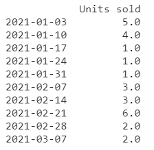
I hope you are able to spot the difference in both cases with the above images.
Linear Interpolation
Linear Interpolation
Time series data has a lot of variations. The above methods of imputing using backfill and forward fill isn’t the best possible solution. Linear Interpolation to the rescue!
Here, the values are filled with incrementing or decrementing values. It is a kind of imputation technique, which tries to plot a linear relationship between data points. It uses the non-null values available to compute the missing points.
interpolated=df.interpolate(limit_direction="both")
print(interpolated)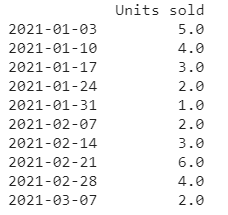
Compare these values to backward and forward fill and check for yourself which is good!
These are some basic ways of handling missing values in time-series data
Algorithms robust to missing values
There are some cases, where none of the above works well. Yet, you need to do an analysis. Then, you should opt for algorithms that support missing values. KNN (K nearest neighbors) is one such algorithm. It will consider the missing values by taking the majority of the K nearest values. The random forest also is robust to categorical data with missing values. Many decision tree-based algorithms like XGBoost, Catboost support data with missing values.
Conclusion
To summarize, the first step is to explore the data and find out what variables have missing data, what is the percentage, and what category does it belong to. After this, you will have a strategic idea of what methods you could try. A helpful tip is to try Imputation with K nearest neighbor algorithm apart from a linear regression model. There are a few more recent methods you could look up like using Datawig, or Hot-Deck Imputation methods if the above methods don’t work.
I hope you liked the read.
You can connect with me at: [email protected]
Linkedin: data pre-processing
The media shown in this article are not owned by Analytics Vidhya and are used at the Author’s discretion.


