Dealing with Missing Values for Data Science Beginners

This article was published as a part of the Data Science Blogathon

Overview

Most data scientists spend their time in data cleaning and preprocessing. Real-world datasets are always challenging.

Before diving into the data, there are a few things I’d want to say, you should know how the data is generated and what features have an impact on the business, only then you can give the best data results. The data results can be visualizations, predictions, or any other analysis related to data. My recommendation is to always ask the business team more questions about data.

In this post, writing about how the data goes missing and what are all the doable ways in which to handle missing values.

Image 1

In the field of data-related research, it is very important to handle missing data either by deleting or imputation(handling the missing values with some estimation).

Well moving forward, when it comes to data science first step while dealing with datasets is data cleaning i.e, handling missing values.

Handling missing values in datasets is necessary?
I say YES! because the data is not complete without handling missing values and many machine learning algorithms do not allow missing values.

Before handling missing values, one should understand why and where data is missing.

D.B.Rubin describes three types of missing data based on the mechanism of missingness.

 

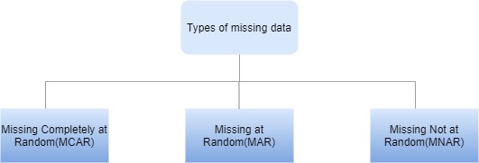
Image by Author

Because these are statistical notions, there hasn’t been much published about them. If you don’t want to know, you can skip the following topics.

Missing Completely at Random(MCAR)

In the dataset, the values are Missing Completely at Random (MCAR) if the events that cause any explicit data item being missing are freelance each of evident variables and of unperceivable parameters of interest, and occur entirely at random. This type of data missing occurs when there is an equipment failure or some design fault.

The main advantage of MCAR is that the analysis is unbiased. Data lost with design fault do not impact other parameters in the model.

Missing at Random(MAR)

It is confusing and better to state it as missing temporarily at random. We can see a connection with other features in the dataset. ​Though, the original values that are missing are random.

Missing at Random is also called Missing Conditionally at Random because the missingness is conditional on another variable.

For example, a registry on patient data may confront data as MAR, where the smoking status is not documented in female patients because the doctor did not want to ask.

Missing not at Random(MNAR)

The missing data model was similar to other features in the data set, but beyond that, the missing data values ​​are not random. If the data is missing in the variable considered then it is said to be missing not at random(MNAR).

Now we move on to the Techniques of Dealing with Missing Values

Image by Author

Handling missing data is not a simple job in the field of data analysis. Approaches may lead to the Good, the Bad, and the Unimaginable.

Some common ways of handling missing values ​​are Deletions and Imputations.

Note: How missing values be in real-world datasets? They can have nan values, empty, constants like -777,999, and in rare cases outliers are also treated as missing and imputed later.

Deletions of Missing Values

Deleting data may be a crucial thing in Machine learning as a result of we tend to find ourselves losing data observations, trends, and patterns from one feature to another.

My recommendation, to get rid of data is not a robust solution for tracking, but sometimes there is a lack of a lot of data observations and that data is not heavily influenced by target variables that we used for the analysis, which means we can choose the Data Deletion Techniques.

Two types of Deletions are

• Listwise Deletions
• Pairwise Deletions

Listwise Deletion

For example,

Consider a model profit (dependent variable) in the table above. On performing listwise deletion Index 1 and 2 rows were removed from the table before analysis.

Cons

When the cause of missing data isn’t random, listwise deletion is another source of concern.

When surveying data the questions in questionnaires aiming to extract sensitive information (eg., income, some medical history).In such cases, folks won’t be revealing the data and ensuing bias in data findings.

Listwise deletion is not a better option in such cases. Imputations are the alternative techniques for eliminating bias when dealing with missing data.

Pairwise Deletion

Pairwise deletion makes an attempt to reduce the loss that happens in listwise deletion.

It calculates the correlation between two variables for every pair of variables to which data is considered. The coefficient of correlation can be used to take such data into account.

The advantage of using pairwise deletion is that it’ll increase power in your analyses. Pairwise deletion is less biased for MCAR or MAR data.

Deleting Columns with Missing Values

Looking into the dataset when there is more than 60% of data is missing most well-liked dropping variables when it involves taking the choice of dropping variable that variable shouldn’t impact overall analysis.

One should check with the business team about the importance of this trait and its implications or to suggest a better substitute for the missing variable instead of dropping it.

Dropping variables is not suggested in several cases as a result of it affects the analysis.

Imputation of Missing Values

Imputation is that the method of substituting missing data with substituted values.

Data is like people–interrogate it hard enough and it will tell you whatever you want to hear.

Two types of Imputations are majorly categorized

• General
• Time-Series

General Data

General data is mainly imputed by mean, mode, median, Linear Regression, Logistic Regression, Multiple Imputations, and constants.

Further General data is divided into two types Continuous and Categorical.

Here we are attending to take one dataset and that we gonna apply some imputation techniques.

Dataset looks like

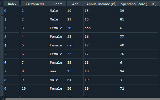
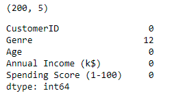
To list the number of missing values ​​in relation to all columns

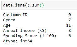
In the above dataset, column names with Genre(categorical ) have 7, Age is11, Annual Income has 8, and Spending Score has 6 missing values. Here we have both categorical and continuous variables to handle.

Good to know, As glorious numerical variables can be continuous or discrete. Before playing imputations, one must be clear with clear with these two types.

Discrete variables are finite with specific range and are countable and are typically whole numbers, such as 1, 2, and 3. Samples of discrete variables like the number of rooms, the number of cars, or the number of bikes. If discrete variables have a large number of levels, it’s advisable to treat them like continuous variables.

Continuous variables are those whose values could take any number at intervals in a range. Samples of continuous variables include the value of a product, salary, house price, height or weight.

Categorical variables are variables that can be a number of possible values and also called labels. Samples of categorical variables like country names, gender, the color of the ball, which takes values of red, green, blue, and so on.

Handling categorical variables

From the above data, column Genre is a categorical variable it has 7 missing values and filling it by constant.

df['Genre'].isna().sum()

7

# Here filling missing values with constant 'NOTKNOWN'
df['Genre'] = df['Genre'].fillna('NOTKNOWN')
df['Genre'].isna().sum()

0

We now predict missing values using Logistic Regression.

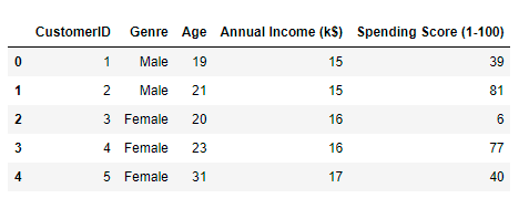
Sample dataset.,

data.head()

print(data.shape)
data.isna().sum()

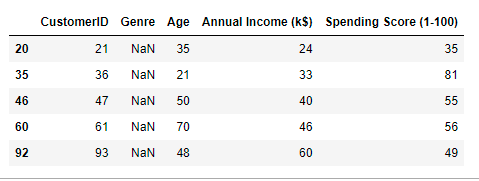
Here we can see 12 missing values in the Genre column.

Separating the missing or nan value rows.

test = data[data['Genre'].isna()]
train = data.dropna()

Let us check test data

test.head()

print(train.shape)
print(test.shape)

(188, 5)

(12, 5)

Preparing data

X_train = train.drop(['Genre'], axis=1)
y_train = train['Genre']
X_test = test.drop(['Genre'], axis=1)

Model

# Getting ready a model to predict missing values(Genre column)
from sklearn.linear_model import LogisticRegression
logistic = LogisticRegression(random_state = 0)
logistic.fit(X_train, y_train)

Predicting the test data

y_pred = logistic.predict(X_test)

After predicting the test data below, the code represents replacing the missing data with predicted values.

Checking the results

print(data.Genre.isna().sum(), "missing values")
data.loc[data['Genre'].isnull(), 'Genre'] = y_pred
print("After imputation")
print(data.Genre.isna().sum(), "missing values")

In some situations replacing mode for categorical variables is additionally a smart idea.

To replace with mode,

data['Genre'] = data['Genre'].fillna(data['Genre'].mode()[0])

Handling Continuous variables

I do know everyone aware of these terms tho’ alittle glance.

Mean is that the average of all the numbers in the dataset.

Mode is that the most commonly occurring value in the dataset.

Median is that the middle value when the data is ordered from least to large.

eg. dataset={1,6,7,7,8,9,5,3}

Mean, average {(1+6+7+7+8+9+5+3)/8} = 5.75

Mode, select the most common value from data {1,6,7,7,8,9,5,3} = 7

Median, arrange data from least to large and choose middle value{1,3,5,6,7,7,8,9} = 6.5

Filling missing values in the Age column.

data['Age'] = data['Age'].fillna(data['Age'].mean()) # filling missing values by mean
data['Age'] = data['Age'].fillna(data['Age'].mode()[0]) # mode
data['Age'] = data['Age'].fillna(data['Age']).median() # median

From the on top of 3 strategies either use anyone kind that suits your dataset.

We use Linear Regression to predict continuous variables.

Similar to the logistic regression we did earlier, one factor I would like to share is the need to check for the correlation between the target variable(here is the missing values column) and other features. If there is no correlation, the predictions goes bad.

Linear Regression to predict missing values.

# Reading data
data = pd.read_csv("sales_data.csv")
# Separating missing or nan values rows
test = data[data['Age'].isna()] # Assume the Age column contains missing values.
train = data.dropna()
# Preparing Data
X_train = train.drop(['Age'], axis=1)
y_train = train['Age']
X_test = test.drop(['Age'], axis=1)
# Getting ready a model to predict missing values(Genre column)
from sklearn.linear_model import LinearRegression
linear = LinearRegression()
linear.fit(X_train, y_train)
# Predictions
y_pred = logistic.predict(X_test)
# filing the missing values with predictions
data.loc[data['Age'].isnull(), 'Age'] = y_pred

Multiple Imputations

All of the strategies presented so far are “single imputation,” which means that each value in the dataset is populated exactly once. Single imputation’s main disadvantage is that, while these algorithms find probable maximum likely values, they do not produce inputs that correctly mimic the underlying data’s distribution.

Of course, If we are prone to making allowances for lacking data,, we could expect some variability: extreme values, outliers, and data sets that do not fully match the “pattern” of the data. The noise is inherent in the data set, but substituting the mean has no effect on how it is represented in your result. As a result, following models that are sensitive to a trend(the presence of the mean in the data set) that is not present in the underlying data will have biases. This successively reduces the accuracy during both the train and test phases.

Here, Multiple imputations are performed using fancyimpute.

Fancyimpute consists of several imputation algorithms. Involves all columns to calculate missing values.

Two main methods we use here to impute missing values

 pip install fancyimpute

K-Nearest Neighbor for Missing Value Imputation

K-NN algorithm stores all the available knowledge and classifies brand new data supported the similarity. this suggests once new data seems then it is often simply classified into a good suite category by exploitation K-NN algorithm.

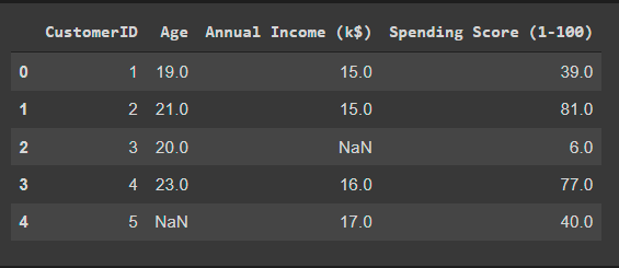
Sample data before imputations.,

data

Applying Knn imputer from fancyimpute,

from fancyimpute import KNN
knn_imputer = KNN()
# imputing the missing value with knn imputer
data = knn_imputer.fit_transform(data)

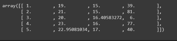
After imputations,

data

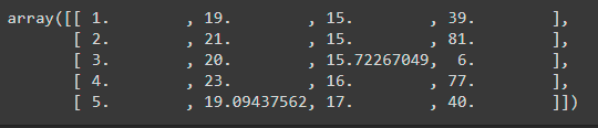
After performing imputations, data becomes numpy array.

Note: KNN imputer comes with Scikit-learn.

MICE or Multiple Imputation by Chained Equation

Multiple Imputation by Chained Equations is a powerful and informative method for dealing with missing values in datasets.

Applying mice imputer

from fancyimpute import IterativeImputer
mice_imputer = IterativeImputer()
# filling the missing value with mice imputer
data = mice_imputer.fit_transform(data)

After imputations,

Note: Multiple imputations have a number of benefits over those alternative missing data approaches.

Time-Series Imputations

Data without trend or seasonality are mostly imputed by mean, median, mode, and random sample imputation.

Data with the trend and without seasonality are mostly imputed by Linear Interpolation.

Data with seasonality and trend is imputed by Seasonal Adjustment with Interpolation.

Random Sample Imputation

To know more about Random sample imputation click here

Interpolation

The method of interpolation is to estimate unknown values by comparing them to known values. Interpolation is commonly used by investors to forecast stock values since it generates new data points from existing data.

There are several types of interpolation techniques

The best example is looking at the stock price data for a year. If we assume that data for a month (July) is missing from this dataset, the data for the month of July is filled by calculating the moving average of June and August. We can use interpolation to calculate the moving average.

Pandas have a function interpolate().

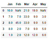
Consider the sample dataset,

data

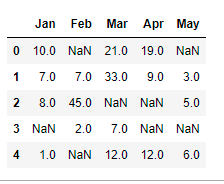
We will use some interpolation techniques.

data.interpolate(method ='linear', limit_direction ='forward')

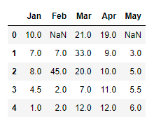
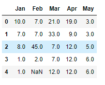
data.interpolate(method ='linear', limit_direction ='backward')

It imputes the nan values in the backward direction.

Note: we can a use limit parameter in interpolate() function to fill the maximum number of consecutive Nan values.

This is the way we use our function to predict the value of the dependent variable for an independent variable found in the data set.

Interpolation is used to cope with data of higher dimensions. To know more about interpolation facilities check here

Imputation by ffill

This ffill method is used to fill missing values by the last observed values.

From the above dataset

data.fillna(method='ffill')

From the output we see that the first line still contains nan values, as ffill fills the nan values ​​from the previous line.

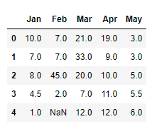
Imputation by bfill

This bfill method is used to fill the missing values with the next observed values.

data.fillna(method='bfill')

From the output we see that the last line still contains nan values, as bfill fills the nan values ​​from the following line. Since there is no next line.

These two methods can also be used by GroupBy function. To know more about groupby filling the missing values, click here .

Time series data show many variations over time. Hence, imputing the use of forward fill and backward fill is not the best possible solution to handle the problem of missing data. A more suitable alternative would be the use of interpolation methods.

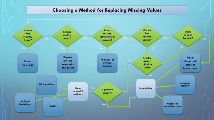
Image 2

Conclusion

Lack of data is a sad reality when it comes to data analysis. We cannot completely avoid situations like this as data scientists need to take several corrective actions to ensure they don’t negatively impact the analytics process.

There is no “perfect” way to fill in the missing data. It just all comes down to the requirement to try and do trials.

Hope you enjoy the content of this post. Thanks for reading!

Image Source:

• Image 1- flickr.com
• Image 2 – datasciencecentral.com