Master the basics of R Programming

This article was published as a part of the Data Science Blogathon

Overview:

• Introduction to the R programming language
• Data Structures available in R: vectors, factors, matrices, lists, data frames
• Overview of conditional statements and functions
• Linear Regression Model

Introduction

R is a programming language created and developed in 1991 by two statisticians at the University of Auckland, in New Zealand. It officially became free and open-source only in 1995. For its origins, it provides statistical and graphical techniques, linear and non-linear models, techniques for time series, and many other functionalities. Even if Python is the most common in the Data Science field, R is still widely used for specialized purposes, like in financial companies, research, and healthcare.

I know that beginning to program with R can be intimidating without any idea where to start. On the web, there are many tutorials that start fastly to explain topics skipping the basics that are needed to understand better the topic. For this reason, I am writing this guide to help you in getting started with R. To have an ordered structure, we need to split this article into building blocks, focusing on one block at a time.

Requirements to Learn R Programming

If you want to start programming in R, you need to install the last versions of R and R studio. You are surely asking yourself why you need to install both. If you prefer, you can install only R and you will have a basic tool to write the code. In addition, R studio provides an intuitive and efficient graphical interface to write code in R. It allows to divide the interface into subwindows to visualize separately the code, the output of the variables, the plots, the environment, and many other features.

Assignment

When we program in R, the entities we work with are called objects [1]. They can be numbers, strings, vectors, matrices, arrays, functions. So, any generic data structure is an object. The assignment operator is <-, which combines the characters < and -. We can visualize the output of the object by calling it:

x <- 23
x
#[1] 23

A more complex example can be:

x <- 1/1+1*1
y <- x^4
z <- sqrt(y)
x
[1] 2
y 
[1] 16
z 
[1] 4

As you can notice, the mathematical operators are the ones you use for the calculator on the computer, so you don’t need the effort to remember them. There are also mathematical functions available, like sqrt, abs, sin, cos, tan, exp, and log.

Vectors in R Programming

In R, the vectors constitute the simplest data structure. The elements within the vector are all of the same types. To create a vector, we only need the function c() :

v1 <- c(2,4,6,8)
v1
# [1] 2 4 6 8

This function simply concatenates different entities into a vector. There are other ways to create a vector, depending on the purpose. For example, we can be interested in creating a list of consecutive numbers and we don’t want to specify them manually. In this case, the syntax is a:b , where a and b correspond to the lower and upper extremes of this succession. The same result can be obtained using the function seq()

v2 <- 1:7
v2
#[1] 1 2 3 4 5 6 7

v3 <- seq(from=1,to=7)
v3
#[1] 1 2 3 4 5 6 7

Output:

[1] 1 2 3 4 5 6 7

The function seq() can also be applied to create more complex sequences. For example, we can add the argument by the step size and the length of the sequence:

v4 <- seq(0,1,by=0.1)
v4
#[1] 0.0 0.1 0.2 0.3 0.4 0.5 0.6 0.7 0.8 0.9 1.0

v5 <- seq(0,2,len=11)
v5
#[1] 0.0 0.2 0.4 0.6 0.8 1.0 1.2 1.4 1.6 1.8 2.0

To repeat the same number more times into a vector, the function rep() can be used:

v6 <- rep(2,3)
v6
v7 <-c(1,rep(2,3),3)
v7

#[1] 2 2 2
#[1] 1 2 2 2 3

There are not only numerical vectors. There are also logical vectors and character vectors:

x <- 1:10
y <- 1:5 
l <- x=y 
l
c <- c('a','b','c')
c

#[1]  TRUE  TRUE  TRUE  TRUE  TRUE FALSE FALSE FALSE FALSE FALSE
#[1] "a" "b" "c"

Factors in R Programming

factors are specialized vectors used to group elements into categories. There are two types of factors: ordered and unordered. For example, we have the countries of five friends. We can create a factor using the function factor()

states <- c('italy','france','germany','germany','germany')
statesf<-factor(states)
statesf
#[1] italy   france  germany germany germany
#Levels: france germany italy

To check the levels of the factor, the function levels() can be applied.

levels(statesf)
#[1] "france"  "germany" "italy"

Matrices in R Programming

As you probably know, the matrix is a 2-dimensional array of numbers. It can be built using the function matrix()

m1 <- matrix(1:6,nrow=3)
m1

#      [,1] [,2]
#[1,]    1    4
#[2,]    2    5
#[3,]    3    6

m2 <- matrix(1:6,ncol=3)
m2

#       [,1] [,2] [,3]
#[1,]    1    3    5
#[2,]    2    4    6

It can also be interesting combine different vectors into a matrix row-wise or column-wise. This is possible with rbind() and cbind() :

countries <- c('italy','france','germany')
age <- 25:27
rbind(countries,age)
#          [,1]    [,2]     [,3]     
#countries "italy" "france" "germany"
#age       "25"    "26"     "27"

or

countries <- c('italy','france','germany')
age <- 25:27
cbind(countries,age)
#     countries age
#[1,] "italy"   "25"
#[2,] "france"  "26"
#[3,] "germany" "27"

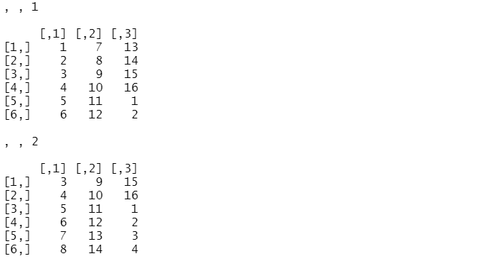
Arrays in R Programming

Arrays are objects that can have one, two, or more dimensions. When the array is one-dimensional, it coincides with the vector. In the case it’s 2D, it’s like to use the matrix function. In other words, arrays are useful to build a data structure with more than 2 dimensions.

a <- array(1:16,dim=c(6,3,2))
a

lists

The list is a ordered collection of objects. For example, it can a collection of vectors, matrices. Differently from vectors, the lists can contain values of different type. They can be build using the function list() :

x <- 1:3
y <- c('a','b','c')
l <- list(x,y)
l

#[[1]]
#[1] 1 2 3 
#
#[[2]]
#[1] "a" "b" "c"

Data frames in R Programming

A data frame is very similar to a matrix. It’s composed of rows and columns, where the columns are considered vectors. The most relevant difference is that it’s easier to filter and select elements. We can build manually the dataframe using the function data.frame() :

countries <- c('italy','france','germany')
age <- 25:27
df <- data.frame(countries,age)
#  countries age
#1     italy  25
#2    france  26
#3   germany  27

An alternative is to read the content of a file and assign it to a data frame with the function read.table() :

df <- read.table('titanic.dat')

Like in Pandas, there are other functions to read files with different formats. For example, let’s read a csv file:

df <- read.csv('titanic.csv')

Like in Python, R provides pre-loaded data using the function data() :

data(mtcars)
head(mtcars)

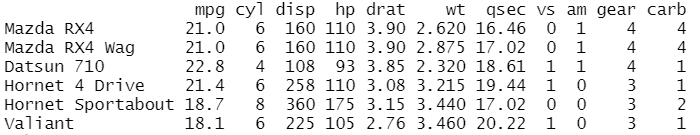
The function head() allows visualizing the first 6 rows of the mtcars dataset, which provides the data regarding fuel consumption and ten characteristics of 32 automobiles. The features are

To check all the information about the dataset, you write this line of code:

help(mtcars)

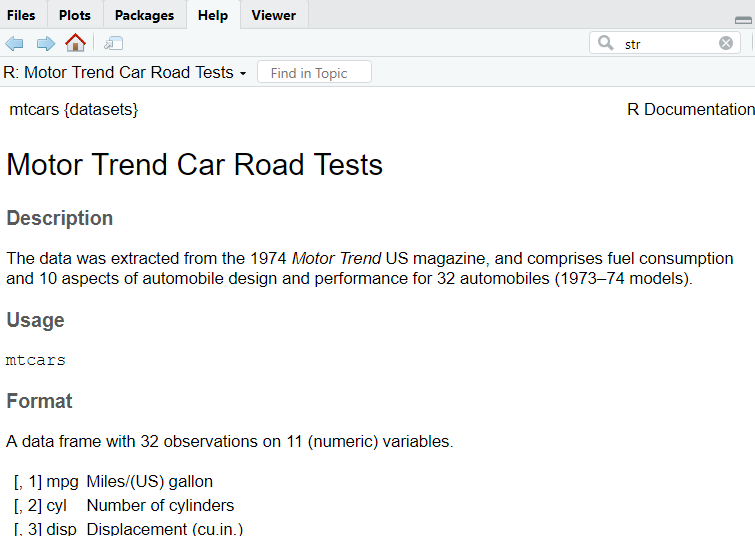
In this way, a window with all the useful information will open. To have an overview of the dataset’s structure, the function str() can allow having additional insights into the data:

str(mtcars)

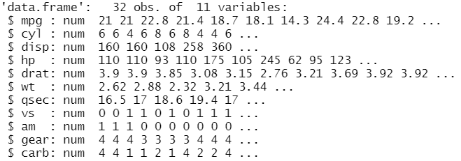
From the output, it’s clear that there are 32 observations and 11 variables/columns. From the second line, there is a row for each variable that shows the type and the content. We show separately the same information using:

• the function dim() to look at the dimensions of the data frame
• the function names() to see the names of the variables

dim(mtcars)
#[1] 32 11
names(mtcars)
[1] "mpg"  "cyl"  "disp" "hp"   "drat" "wt"   "qsec" "vs"   "am"   "gear" "carb"

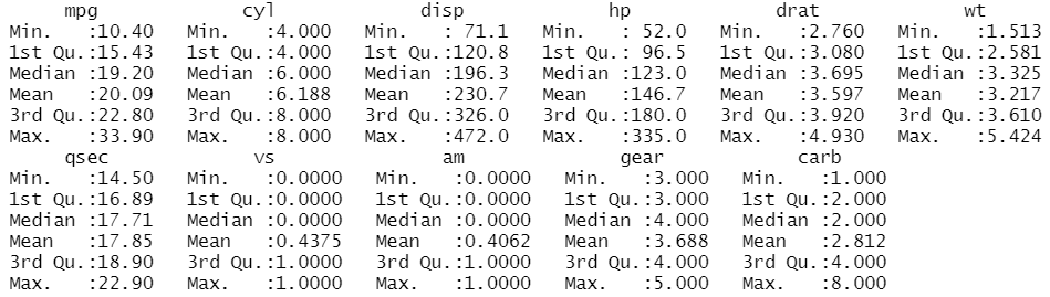
The summary statistics of the variables can be obtained through the function summary()

summary(mtcars)

We can access specific columns using the expression namedataset$namevariable. If we want to avoid specifying every time the name of the dataset, we need the function attach().

mtcars$mpg
# [1] 21.0 21.0 22.8 21.4 18.7 18.1 14.3 24.4 22.8 19.2 17.8 16.4 #17.3 15.2 10.4 10.4 14.7 32.4 30.4
#[20] 33.9 21.5 15.5 15.2 13.3 19.2 27.3 26.0 30.4 15.8 19.7 15.0 #21.4
attach(mtcars)
mpg
# [1] 21.0 21.0 22.8 21.4 18.7 18.1 14.3 24.4 22.8 19.2 17.8 16.4 #17.3 15.2 10.4 10.4 14.7 32.4 30.4
#[20] 33.9 21.5 15.5 15.2 13.3 19.2 27.3 26.0 30.4 15.8 19.7 15.0 #21.4

In this way, we attach the data frame to the search path, allowing to refer to the columns with only their names. Once we attached the data frame and we aren’t interested anymore to use it, we can do the inverse operation using the function detach().

We can also try to select the first row in the data frame using this syntax:

mtcars[1,]

Note that the index starts from 1, not from 0! If we want to extract the first columns, it can be done in this way:

mtcars[,1]
#[1] 21.0 21.0 22.8 21.4 18.7 18.1 14.3 24.4 22.8 19.2 17.8 16.4 #17.3 15.2 10.4 10.4 14.7 32.4 30.4
#[20] 33.9 21.5 15.5 15.2 13.3 19.2 27.3 26.0 30.4 15.8 19.7 15.0 #21.4

We can also try to filter the rows using a logical expression:

mtcars[mpg>20,]

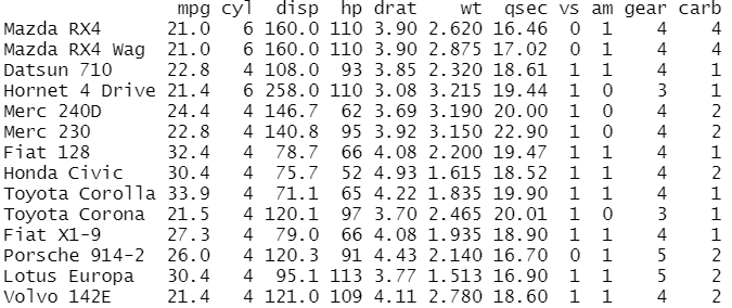
we can also specify the column while we filter:

mtcars[mpg>20,'mpg']
#[1] 21.0 21.0 22.8 21.4 24.4 22.8 32.4 30.4 33.9 21.5 27.3 26.0 30.4 21.4

For and While in R Programming

The for loop is used to iterate elements over the sequence like in Pandas. The difference is the addition of the parenthesis and curly brackets. It has slightly different syntax:

for (var in seq) statement

for (i in 1:4) 
{print(i)}
#[1] 1
#[1] 2
#[1] 3
#[1] 4

while executes a statement or more statements as long as the condition is true

while (cond) statement

i<-1
while (i<6)
{print(i)
  i<-i+1}

#[1] 1
#[1] 2
#[1] 3
#[1] 4
#[1] 5

I statement in R Programming

The syntax of the if statement is similar to the one in Python. As before, the difference is the addition of the parenthesis and curly brackets.

if (cond1) {statement1} else {statement2}

and

if (cond1) {statement1} else if {statement2} else {statement3}

for (i in 1:4)
{if (i%%2==0) print('even') else print('odd')
}
#[1] "odd"
#[1] "even"
#[1] "odd"
#[1] "even"

If we want to compare two numbers and see which number is greater of the other, we can do it in this way:

a <- 10
b <- 2
if (b > a){
  print('b is greater than a')
}else if (a == b){
  print('a and b are equal')
}else {
  print('a is greater than b')
  }
# [1] "a is greater than b"

There is also a vectorized version of the if statement, the function ifelse(condition,a,b) . It’s the equivalent of writing:

if condition {a} else {b}

For example, let’s check if a number is positive:

x<-3
ifelse(x>=0,'positive','negative')
# [1] "positive"

Function in R Programming

The function is a block of code used to perform an action. It runs only when the function is called. It usually needs parameters, that need to be passed, and returns an output as result. It’s defined with this syntax in R:

namefunction <- function(par_1,par_2,…)

{expression(s)}

Let’s create a function to calculate the average of a vector:

average <- function(x)
{ val = 0
  for (i in x){val=val+i}
  av = val/length(x)
  av
    }

average(1:3)
#[1] 2

Probability distributions in R Programming

A characteristic of R is that it provides functions to calculate the density, distribution function, quantile function and random generation for different probability distributions. For example, let’s consider the normal distribution:

• dnorm(x) calculates the value of the density in x
• pnorm(x) calculates the value of the cumulative distribution function in x
• qnorm(p) calculates the quantile of level p
• rnorm(n) generates a sample from a standard normal distribution of n dimension

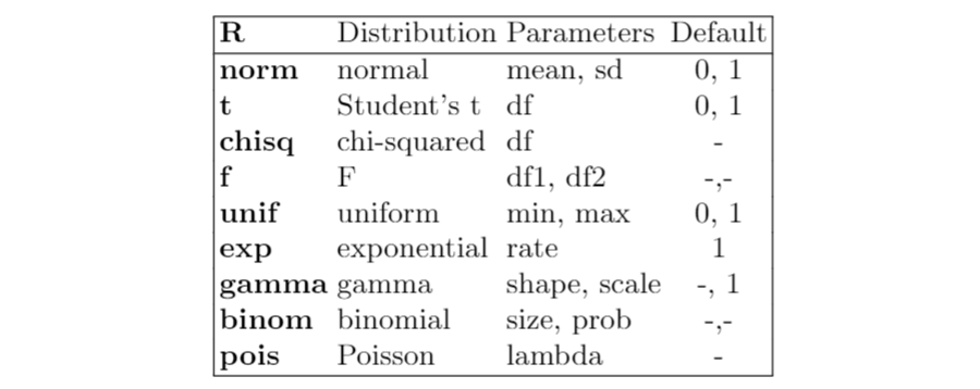
Now, I show a table with the most known distributions available in R:

Plotting commands in R Programming

The graphs are very important to get insights into the data. R provides plotting commands to display a huge variety of plots:

• plot(x) is the most common function used to produce scatterplots
• pairs(X) is used to display multivariate data. It produces a pairwise scatterplot matrix of the variables contained in X.
• hist(x) is used to display the histogram
• box(x) is used to display the boxplot
• qqplot(x) is used to produce the Q-Q plot, useful to check if the distribution analyzed is normal or not.
• abline(h=y) and abline(v=x) are the most used function to add horizontal and vertical lines in the already built plot
• curve(expr,add=FALSE) is used to display a curve, that can be added or not to an already existing graph.
• par(mfrow=(r,c)) is used put multiple graphs in a single plot. The mfrow parameter specifies the number of rows and the number of columns.
• legend(x,y,legend,...) is used to specify the legend in the plot at the specified position (x,y)

For example, we can generate a sample with 200 units from a normal distribution. Let’s suppose we don’t know the distribution and we want to display the histogram and the boxplot:

x <-rnorm(200)
par(mfrow=c(1,2))
hist(x,ylim=c(0,0.5),prob=TRUE)
curve(dnorm(x),add=TRUE)
boxplot(x)

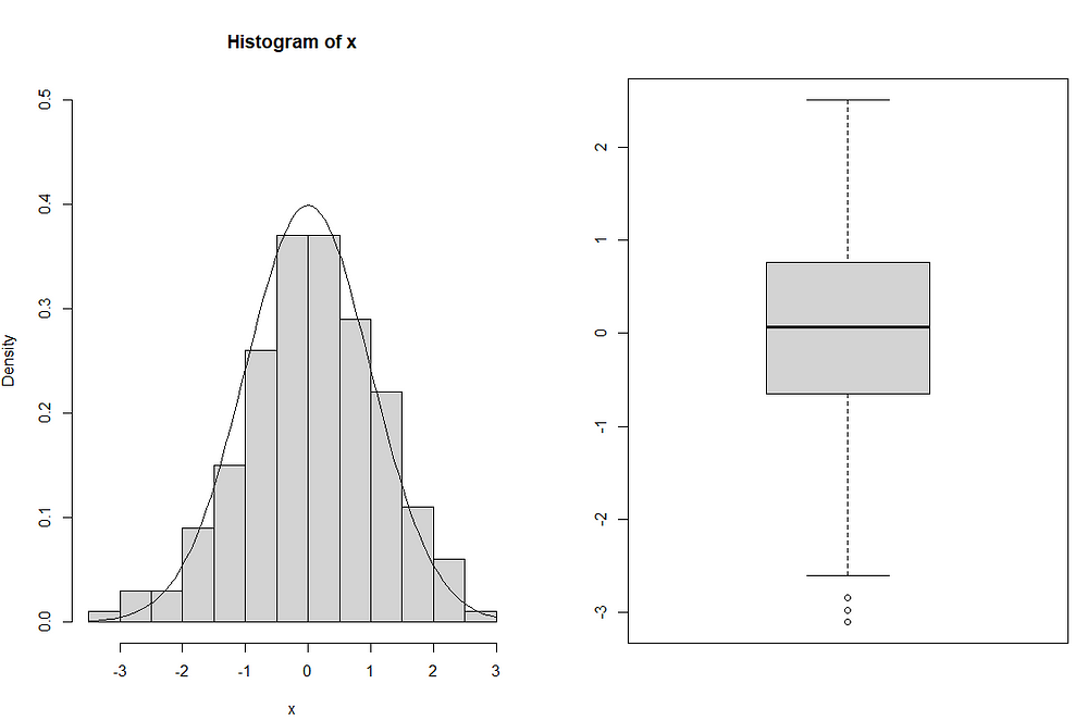
Since the sample size is high, the histogram appears similar to a normal density curve, as shown in the figure. From the boxplot, it can be seen that the distribution is symmetric and there are three outliers that have lower values than the minimum.

Linear Regression in R

The models of linear regression are the most widely known models that want to predict a real-valued output Y [2]. It has the following form:

When there is more than one predictor, the model is called Multiple Linear Regression. It’s characterized by two advantages: simplicity and high interpretability. Simplicity because it’s based on few assumptions that need to be respected to work well:

• normality of the response variable Y
• a linear relationship between the mean of the response variable and the dependent variables. Indeed, the coefficients βj can be interpreted as the average effect on the response variable Y of one unit increase in the dependent variable, corresponding to the coefficient considered, while fixing the values of all the other predictors.
• homoscedasticity of the response variable

Moreover, it allows to study the strength and the relationship between the variables, providing more insights into the data. In the model, βj are unknown parameters and need to be estimated through the ordinary least squares method (OLS), by minimizing the sum of squared residuals:

Another important aspect is the hypothesis test, which allows checking if there is a relationship between the response and the predictor xj. This is possible testing the null hypothesis, called in this way because it tests if the coefficient βj is equal to 0, and, then, calculating the standardized coefficient:

There is also another test used to assess the significance of many coefficients at the same time: H₀: β₁ = … = βp = 0 against the hypothesis that at least one coefficient is non-zero. In this case, the F statistic is used:

Let’s take again the mtcars dataset and let’s suppose that we want to perform the linear regression to see the estimated coefficients. As the first trial, I include only one dependent variable, the number of cylinders in the model, which is called linear regression. The syntax of the formula within the function lm is response~terms, where the response is the response variable, while terms refer to one or more dependent variables included in the model.

data(mtcars)
attach(mtcars)
lm1 <- lm(mpg~cyl)
lm1$coefficients
#(Intercept)         cyl 
#   37.88458    -2.87579

Looking at the parameter of cyl, we can understand that there is negative relationship between the number of cylinders and mpg. To better understand, we can visualize the scatterplot between the two features:

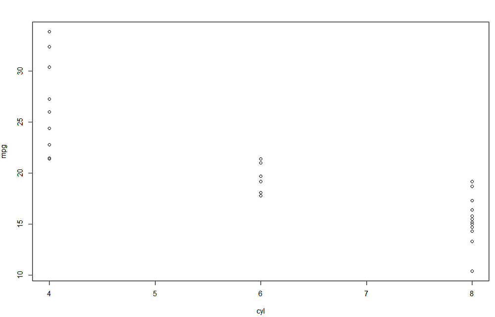
It seems that increasing the number of cylinders lead to a decrease miles/(US) gallon. The most relevant results of the linear model are provided using the function summary() .

summary(lm1)

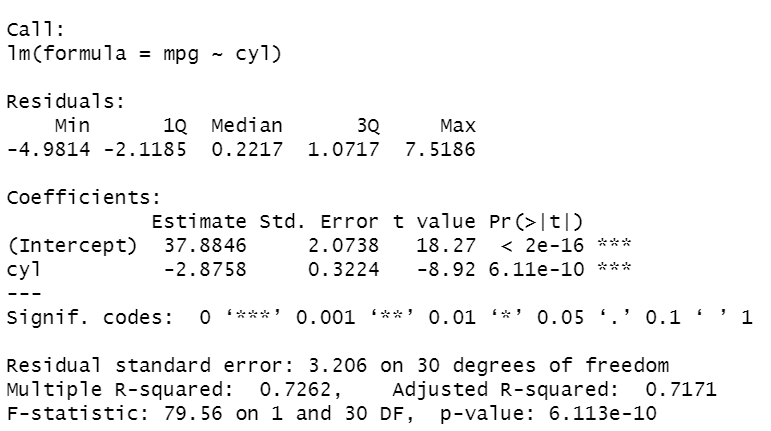
It’s the summary of the results obtained performing the linear regression model on the data. At the top of the output, we can see the variables included in the model. There are some statistics (minimum, first and third quartiles, median, maximum) regarding the residues of the estimated model. After, there is a table containing the estimated coefficients of the model, where each row corresponds to a coefficient. Each row has the following information:

• the value of the estimated coefficient
• the standard Error
• the observed t-value
• the observed level of significance: in case it’s smaller than 0.05, the parameter is significant and, then, there is a linear relationship between that variable and the response variable.

We can see that both coefficients are significant with p-value<0.05 and R² is high, near 1, considering that we only included a variable. cyl’s coefficient is negative and, then, indicates the decrease of value for each increase of one unit in mpg.

We can also try to include another predictor and include the interaction term between cyl and disp:

lm2 <- lm(mpg ~ cyl+disp+cyl:disp)
lm2 <- lm (mpg ~ cyl*disp)
summary(lm2)

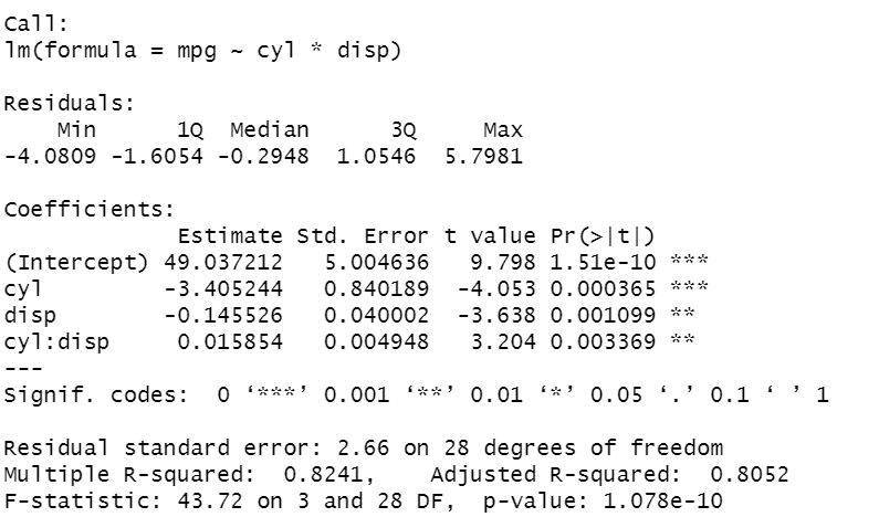
In the code, I show different syntax formats, that allow reaching the same results. Putting the *, between the two features enables to write less code. As before, all the coefficients are significant. Now, the R² is higher, equal to 0.8. To evaluate how well the model explains well the behaviour of the data, an efficient way is to display the residuals versus the fitted values, where the residuals are the differences between the true values and the fitted values.

plot(lm2)

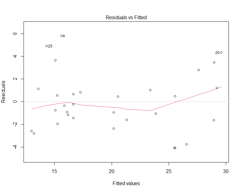
The red curve corresponds to the smooth fit to the residuals and has a U-shape, indicating that there are non-linear associations in the data.

After this step, we can finally predict mpg on new data using the fitted model:

newdata <-data.frame(mpg=20,cyl=8,disp=150,hp=100,drat=3,wt=2.4,
qsec=17,vs=1,am=1,gear=4,carb=2)
predict(lm2,newdata)
#       1 
#18.99105

The summary() needs two parameters, the fitted linear model and the new data, that should be a data frame object. The output shows that the new car is expected to have an mpg value equal to 18.9.

Frequently Asked Questions

Final thoughts

I hope you found useful this guide in programming in R. Starting from the basics, you will be able to perform any type of analysis on the data. As the last topic, I covered linear regression to show the most simple example of data modelling in R. I didn’t split the dataset into training and test sets since the dataset was too small, but you can try it on a bigger dataset. Below, there are some books you can read with many examples in R. Thanks for reading. Have a nice day!

The media shown in this article are not owned by Analytics Vidhya and are used at the Author’s discretion