This article was published as a part of the Data Science Blogathon.
We know how useful convolutional neural networks are. CNNs have transformed image analytics. They are the most widely used building blocks for solving problems involving images. Many architectures like ResNet, Google Net have achieved exceptional accuracies in image classification tasks are built with CNNs. But… These too come with some flaws and one of them is the time they take to train on huge datasets. Separable Convolutions are helpful to tackle this problem.
Conventional Convolution
Let’s understand Conventional Convolution first.
According to Wikipedia convolution is a mathematical operation on two functions that produces a third function that expresses how the shape of one is modified by the other.
A 2D Convolution is a mathematical process in which a 2D kernel slides over the 2D input matrix performing matrix multiplication with the part that is currently on and then summing up the result matrix into a single pixel. You can read more about this here.
What are Separable Convolutions?
A Separable Convolution is a process in which a single convolution can be divided into two or more convolutions to produce the same output. A single process is divided into two or more sub-processes to achieve the same effect. Let’s understand Separable Convolutions, their types in-depth with examples.
Mainly there are two types of Separable Convolutions
- Spatially Separable Convolutions.
- Depth-wise Separable Convolutions.
Spatially Separable Convolutions
In images height and width are called spatial axes. The kernel that can be separated across spatial axes is called the spatially separable kernel. The kernel is broken into two smaller kernels and those kernels are multiplied sequentially with the input image to get the same effect of the full kernel.
For example
(The above-mentioned example is called the Prewitt kernel. This kernel is used to detect edges in the images)
Convolutions with spatially separable kernels
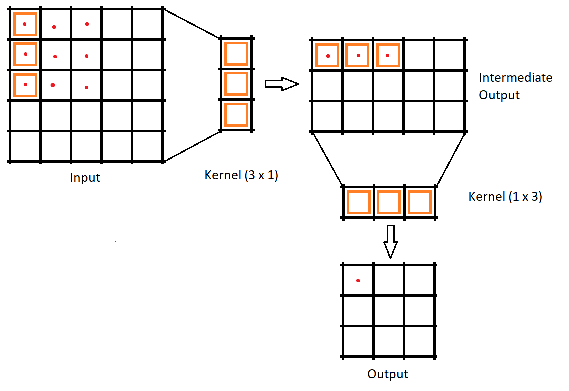
In the conventional convolutions, if the kernel is 3 x 3 then the number of parameters would be 9. In spatially separable convolution we divide the kernel into two kernels of shapes 3 x 1 and 1 x 3. The input is first convolved with 3 x 1 kernel and then with 1 x 3, then the number of parameters would be 3 + 3 = 6. So less matrix multiplication is required.
An important thing to note here is that not every kernel can be separated. Because of this drawback, this method is used lesser compared to Depthwise separable convolutions.
Depthwise Separable Convolutions
When you call tf.keras.layers.SeparableConv2D you would be calling a Depthwise separable convolution layer itself. Here you can use even those kernels which can not be spatially separable. Similar to spatial convolution, here also a regular convolution is divided into two convolutions namely
- Depthwise convolution
- Pointwise convolution
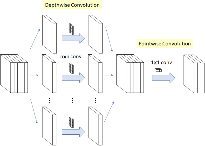
Image credit Imran Junejo
Depthwise convolution
Let us assume we have an image input of shape 7x7x3. We make sure after the depthwise convolution the intermediate image has the same depth. This is done by convoluting with 3 kernels with shape 3x3x1. Each kernel iterates on only one channel of the image-producing an intermediate output of shape 5x5x1 which are stacked together to create an output of shape 5x5x3.
Pointwise convolution
After the depthwise convolution, we have an intermediate output of shape 5x5x3. Now we need to increase the depth of the output, which is done by convoluting with a kernel with shape 1x1xdepth which is called a pointwise convolution. Let us assume the depth is 32. Then after pointwise convolution, the output would have the shape 5x5x32. Which is equivalent to convolution with 32 filters of shape 5×5.
In this example, the regular convolution would have to do 32 3x3x3 kernels that move 5×5 times that is 21600 multiplication but in this method, we would have to do 3x3x3x5x5 + 32x1x1x3x5x5 = 3075 multiplication. So we can see that this method can eliminate a large chunk of multiplication.
Let’s do some hands-on and compare the performances
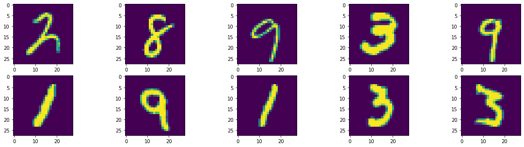
In this explanation, I have taken the most famous mnist dataset. You can know more about this dataset here.
Visualizing random images from the dataset
plt.figure(figsize=(20,5))
for i in range(1,11):
  plt.subplot(2,5,i)
  plt.imshow(x_train[randint(1,60000)].reshape(28,28))
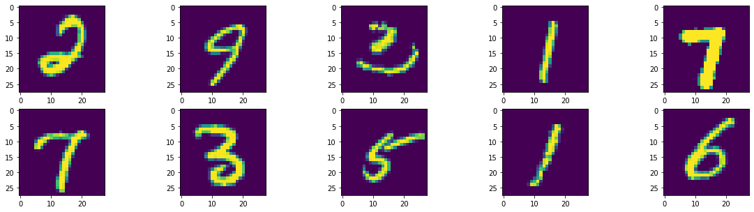
plt.figure(figsize=(20,5))
for i in range(1,11):
  plt.subplot(2,5,i)
  plt.imshow(x_test[randint(1,10000)].reshape(28,28))
Model with Conventional CNNs
model = tf.keras.Sequential([
        tf.keras.layers.Conv2D(8, 7, input_shape=(28,28,1), strides=2),
        tf.keras.layers.Conv2D(16, 5, strides=2),
        tf.keras.layers.Conv2D(32, 3),
        tf.keras.layers.GlobalAveragePooling2D(),
        tf.keras.layers.Dense(10, activation='softmax')
])
model.compile(loss='categorical_crossentropy', metrics=['acc'])
model.summary()
Model: "sequential_17"
_________________________________________________________________
 Layer (type)                Output Shape              Param #
=================================================================
 conv2d_43 (Conv2D)          (None, 11, 11, 8)         400

 conv2d_44 (Conv2D)          (None, 4, 4, 16)          3216

 conv2d_45 (Conv2D)          (None, 2, 2, 32)          4640

 global_average_pooling2d_17  (None, 32)               0
  (GlobalAveragePooling2D)

 dense_17 (Dense)            (None, 10)                330

=================================================================
Total params: 8,586
Trainable params: 8,586
Non-trainable params: 0
_________________________________________________________________
Conventional model’s performance
model.save("model.hdf5")
size = os.path.getsize('model.hdf5')
print('Size of file is', size/1024, 'kilo bytes')
t = time()
loss, acc = model.evaluate(x_test, y_test)
print('Test Accuracy = {}'.format(acc))
print('Time taken for evaluation of 10000 images = {:.2f} seconds'.format(time()-t))
Size of file is 105.2265625 kilo bytes
313/313 [==============================] - 1s 3ms/step - loss: 0.2982 - acc: 0.9169
Test Accuracy = 0.9168999791145325
Time taken for evaluation of 10000 images = 1.43 seconds
Model with Depth-wise CNNs
I kept all the other parameters exactly same and replaced Conv2D with SeparableConv2D
model = tf.keras.Sequential([
        tf.keras.layers.SeparableConv2D(8, 7, input_shape=(28,28,1), strides=2),
        tf.keras.layers.SeparableConv2D(16, 5, strides=2),
        tf.keras.layers.SeparableConv2D(32, 3),
        tf.keras.layers.GlobalAveragePooling2D(),
        tf.keras.layers.Dense(10, activation='softmax')
])
model.compile(loss='categorical_crossentropy', metrics=['acc'])
model.summary()
Model: "sequential_18"
_________________________________________________________________
 Layer (type)                Output Shape              Param #
=================================================================
 separable_conv2d_9 (Separab  (None, 11, 11, 8)        65
 leConv2D)

 separable_conv2d_10 (Separa  (None, 4, 4, 16)         344
 bleConv2D)

 separable_conv2d_11 (Separa  (None, 2, 2, 32)         688
 bleConv2D)

 global_average_pooling2d_18  (None, 32)               0
  (GlobalAveragePooling2D)

 dense_18 (Dense)            (None, 10)                330

=================================================================
Total params: 1,427
Trainable params: 1,427
Non-trainable params: 0
_________________________________________________________________
Separable CNN’s performance
model.save("model.hdf5")
size = os.path.getsize('model.hdf5')
print('Size of file is', size/1024, 'kilo bytes')
t = time()
loss, acc = model.evaluate(x_test, y_test)
print('Test Accuracy = {}'.format(acc))
print('Time taken for evaluation of 10000 images = {:.2f} seconds'.format(time()-t))
Size of file is 56.9375 kilo bytes
313/313 [==============================] - 1s 3ms/step - loss: 0.3394 - acc: 0.9021
Test Accuracy = 0.9021000266075134
Time taken for evaluation of 10000 images = 1.11 seconds
Observations
- The number of trainable parameters in Separable CNNs (1.5k) is 82% lesser than Conventional CNNs (8.5k)
- The size of the Model with Separable CNNs (56 KB) is almost half of that of the Model with Conventional CNNs (105 KB)
- Time taken to evaluate 10000 images by the Model with Separable CNNs (1.11s) is almost 23% lesser than that of the Model with Conventional CNNs (1.43s)
- The accuracy of the Model with Separable CNNs (90.2%) is lesser than that of the Model with Conventional CNNs (91.6%)
Drawbacks of Separable Convolutions
We have seen how separable convolutions are useful still we don’t use them very often and the reasons for that are
- Not every kernel can be divided into two kernels in the case of Spatially Separable Convolutions
- As the number of parameters in separated convolutions is lesser we would lose some accuracy.
- Models with Separable convolutions tend to underfit.
- When the model itself is very small reducing the parameters may lead to complete failure of the model.
Conclusion
Separable convolutions are great when you are optimizing the model for smaller size or higher speed compromising least with accuracy. It is not advised to use it when you are optimizing the model for accuracy. Many deep learning algorithms are built using Separable convolutions, one among them is the Xception algorithm which you can go and check out.
You can access the colab link for the above codes here
You can connect with me here
Thank you so much for reading this article. Your feedback is very precious, you share your thoughts on this here.
The media shown in this article is not owned by Analytics Vidhya and are used at the Author’s discretion


