This article was published as a part of the Data Science Blogathon.
Overview. Regression analysis is used to solve problems of prediction based on data statistical parameters. In this article, we will look at the use of a polynomial regression model on a simple example using real statistic data. We will analyze the relationship between the price of gas and its consumption in the United States using the R programming language.
Keywords: polynomial model, regression analysis, Least Squares Method.
What is regression analysis used for?
Regression analysis is used to solve problems of prediction based on data statistical parameters. Such tasks arise, for example, when data is usually obtained from the measurements of economic processes. The task of regression analysis is to select mathematical models that best describe statistical data.
One of the widely distributed common regression analysis models is polynomial regression. This type of model is used to model non-linear statistical relationships between variables. Hence, for instance, a typical problem of polynomial regression in economics is the problem of analyzing costs from the volume of production, demand from the price of products, etc.
Let us look at the use of a polynomial regression model on a simple example using real statistic data. We will analyze the relationship between the price of gas and its consumption in the United States. Statistical data are available for free at the link-
https://www.bp.com/content/dam/bp/business-sites/en/global/corporate/xlsx/energy-economics/statistical-review/bp-stats-review-2021-all-data.xlsx [1]. We will use the R language as the programming language.
Regression analysis steps
It is generally accepted that the steps of regression analysis consist of:
- Formulation or statement of the problem;
- Identifying variables;
- Collection of statistical data;
- Specification of the regression function;
- Estimation of the regression function;
- Evaluation of the accuracy of regression analysis
Statement of the problem
Our task is to find out how US Natural Gas Consumption (Exajoules) vary with the Price change. According to [1] we have a big stock of data about all world energy sources in one file of “xlsx” format. Therefore, we chose US Natural Gas Consumption (Exajoules) and then we extract the information about prices for available years and create our own data source file “US_Natural_gas_consumption.xlsx”.
Identifying variables
Our source file “US_Natural_gas_consumption.xlsx” provides information on the amount of Natural Gas: Consumption (Exajoules) and Price (US dollars per million Btu). In this case, our goal is to predict gas consumption depending on the price, which means that Consumption is the dependent variable Y; and the explanatory variable, in this case, will be Price, i.e. regressor.
Collection of statistical data
Since the original data is collected in xlsx format, we use the “readxl” library:
library(readxl)
data<- read_excel("US_Natural_gas_consumption.xlsx")
str(data)
 $ Year       : num [1:32] 1989 1990 1991 1992 1993 ...
 $ Consumption: num [1:32] 32.2 32.9 34.3 34.3 33.5 ...
 $ Price      : num [1:32] 1.7 1.64 1.49 1.77 2.12 ...
The first six lines of our input data are presented in Table 1.
Table 1
| Year | US Natural Gas: Consumption, (Exajoules) | Price, (US dollars per million Btu) |
| 1989 | 32.24012 | 1.696667 |
| 1990 | 32.91175 | 1.638333 |
| 1991 | 34.27518 | 1.486667 |
| 1992 | 34.2631 | 1.771667 |
| 1993 | 33.50489 | 2.120833 |
| 1994 | 32.79064 | 1.92 |
Regression function specification
We have the simplest case with only two variables therefore the relationship between the values can be represented graphically, which allows choosing the best form of the regression model visually. For this purpose, we create the scatterplot (plot of the points) of the selected variables. Hence, we will use the “ggplot2” library.
library(ggplot2)
graph<-ggplot(data, aes(x=Price, y=Consumption))+
geom_point(size=4)+
labs(x = "Pricesn(US dollars per million Btu)",
     y = "Consumptionn(exajoules)")+
theme_bw()+theme(axis.line = element_line(colour="black"))
graph
The obtained graph is represented in Figure 1.
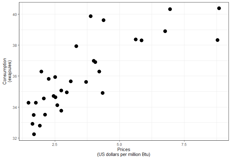
Figure.1. Scatterplot of the US Natural Gas: Consumption vs Price
Based on Fig. 1. we hypothesize about the polynomial nature of the relationship between the variables and add to our graph a fitted line with the following code:
graph + geom_point(colour="grey") + stat_smooth(formula = y ~ poly(x, 1, raw = TRUE))
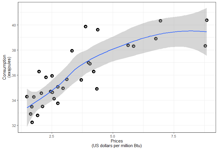
Figure.2. Scatterplot of the US Natural Gas: Consumption vs Price with fitted line.
According to Fig.2, a polynomial function is appropriate to describe our statistical data. Then a theoretical model of polynomial regression is:
Y=β0+β1X+β2X2+β3X3+…+βmXm, (1)
where
Y – is a dependent or predicted variable;
Х – is an independent variable or so-called regressor or predictor;
βm– model parameters.
Based on Fig. 2, we define the degree of polynomial regression. It is enough to be a parabola and the theoretical model of the dependence of the US Natural Gas Consumption from Prices will take the form:
Y=β0+β1X+β2X2 (2)
or in our case
Consumption=β0+β1Price+β2Price2 (3)
Then the empirical (obtained as a result of the experiment) regression function will have the form:
Yi*=β*0+β*1X+β*2X2+ei , (4)
where Yi*– predicted gas consumption, i=1,2,3,…n;
β*m– statistical estimates of
model parameters, m=0,1,2;
ei – error or accidental deviations, i=1,2,3,…n;
n – number of observations.
In our case, the empirical polynomial regression equation looks like this:
Consumption*=β*0+β*1Price+β*2Price2 (5)
So we are faced with the next problem: how, based on the mentioned above statistical data (xi,yi) find such statistical estimates β*m for the unknown parameters βm to get the best possible empirical regression function (5). And so that the plotline of this function should be placed as close as possible to the points (xi,yi) on the entire scatterplot. A measure of the quality of the found statistical estimates β*m and hence the entire empirical function can be estimated by the size of deviations ei , with respect to the empirical line.
Estimation of the Polynomial Regression function
Therefore we conclude that the deviations of real values (xi,yi) from the empirical function (4) were minimal. Then the estimates for the coefficients β*m can be determined by minimizing the sum of the squares of the deviations:

Calculation of the statistical estimates of the model parameters β*m by the criterion of minimization sum of squared errors (6) has the name Least Squares Method.
Least Squares Method for Polynomial Regression
In the case of applying the Least Squares Method to find estimates of model parameters, certain conditions must be met:
1) Expected value (average) of errors ei should be zero: M(ei)=0, i=1,2,3,…n.
This condition requires that random deviations generally do not affect the dependent variable Y. In each particular observation, the deviation ei can take positive or negative values, but there should be no systematic bias of deviations, i.e. they should not be most of the same sign.
2) Variation of random deviations ei should be constant: Var(ei)=ϭ2e(ei)= ϭ2e=const, i=1,2,3,…n.
This condition means that although the random variation may be small or large for each particular observation, this should not be an a priori cause (i.e. reasons that are not based on the experiment), which would cause a large error. Models for which this condition is satisfied are called homoscedastic, and for which it is not – heteroscedastic.
3) Random errors ei and ej (i≠j) must be independent of one another, i.e. do not auto correlate. The fulfillment of this condition assumes that there is no systematic relationship between any random deviations, i.e. the magnitude and sign of any accidental deviation is not the cause of the magnitude and sign of any other accidental deviation.
4) Random errors ei must be independent of the explanatory variables X.
5) Random errors ei must have a normal distribution: ei~N(0,ϭe).
6) The created model should be linear with respect to the parameters. If the dependent variable linearly relates to the independent variable, then this will mean that there is no relationship between the deviations and the predicted (values).
Taking into account the above-mentioned conditions, let us proceed to the estimation of the model parameters by the Least Squares Method. Obviously, a polynomial model can be represented as a special case of a linear model, and therefore, to find statistical estimates of the model parameters, it is sufficient to use the built-in function lm ():
PolynomMod <- lm(Consumption ~ Price+I(Price^2), data=data)
Estimation of the accuracy of the Regression Analysis
Thus, move on to listing the resulting model using the summary () command:
Summary(PolynomMod)
Call:
lm(formula = Consumption ~ Price + I(Price^2), data = data)
Residuals:
    Min      1Q  Median      3Q     Max
-2.4982 -0.8577 -0.2069  0.9235  2.9668
Coefficients:
                    Estimate   Std. Error t value             Pr(>|t|)
(Intercept)  30.1042     1.0471  28.749 < 0.0000000000000002 ***
Price            2.2809     0.5159    4.421             0.000126 ***
I(Price^2)   -0.1383     0.0518  -2.669             0.012324 *
---
Signif. codes:  0 ‘***’ 0.001 ‘**’ 0.01 ‘*’ 0.05 ‘.’ 0.1 ‘ ’ 1
Residual standard error: 1.256 on 29 degrees of freedom
Multiple R-squared:  0.7246,    Adjusted R-squared:  0.7056
F-statistic: 38.15 on 2 and 29 DF,  p-value: 0.000000007573
Consider the results of the listing. The Estimate column shows the estimated parameters of the model, i.e.: β*0=30.1042, β*1=2.2809, β*2=-0.1383.
Then the equation (5) can be represented as:
Consumption*=30.1042+2.2809Price-0.1383Price2
Thus, at zero gas Prices, Consumption will stay at the level of 30.1042, i.e. we can say that regardless of Price changes, gas Us Natural Gas Consumption will be at the level of 30.1042 exajoules. In this case, the constant at 30.1042 exajoules is a starting point of US Gas Consumption. Further, with an increase in price per unit (US dollars per million Btu), Consumption will increase by 2.39870 exajoules, and with an increase in the squared gas Price per unit, Consumption will fall by 0.1383 exajoules. As a conclusion, we estimate that it takes about 2.2809 exajoules more for each additional US dollar in Price (linear effect parameter). Otherwise, the Consumption will decrease by about 0.1383 exajoules per unit of change in Squared Price (quadratic effect parameter).
Column Std.Error shows the standard error of the statistical estimates of model parameters Sβm.
The next column t value relates to the Test of the Significance of the Independent Variables. Suppose we have found the model is significant. Now, we to find if the individual independent variables are significant. This question can be resolved by putting a null hypothesis about the equality to zero of the theoretical coefficient βm (not significant) and the alternative hypothesis that it is not equal to zero (significant). It can be written as follows:
H0: βm=0, Hα: βm≠0.
Then we use the t-test, given by
tm= βm/ Sβm (8)
The calculated t-test equation (8) is shown in the t-value column. It should be compared to the critical values of the tabulated t-distribution with n − m – 1 degree of freedom at significance level α=0.05 (in our listing). Thus, if tm exceeds the critical value then the independent variable is said to be statistically significant.
Equivalently, the p-value of equation (8) would then be less than α. Column Pr(>|t|) shows that all parameters of the model are statistically significant (p < 0.001).
Residual standard error
It is an estimate of Se or average consumption prediction error is essentially the standard deviation of the residuals and equals 1.256. Thus we can say that about two-thirds of the predictions of natural gas consumptions should lay within one standard error or 1.256 exajoules.
Multiple R-squared (the coefficient of determination)
It is a measure of goodness of fit. This goodness-of-fit measure shows how much of variation of the dependent variable is explained by our obtained model. Therefore, variable Price is able to explain only 72.46% of the variation in the Consumption variable. There is (1-0.7246)*100%=27.54% of the variation left unexplained.
Adjusted R-squared
It is a measure that adjusts R-squared for the number of independent variables in equation (5).
F-statistic
It is a test that corresponds to that all coefficients of the independent variables are zero. The alternative is that at least one of these coefficients is not zero. If the F – statistic number is small, the explained variation is small compare to the unexplained variation. Otherwise, if the F-statistic number is big, the explained variation is bid versus the unexplained variation, and we can have a conclusion about the explanatory quality of the created model. The F – statistic number has an associated p-value. If it is sufficiently small, for instance, less than 0.05, then the whole equitation has explanatory power.
Number 29 in our case is called the degrees of freedom (df), which is equal to the number of observations minus the number of estimated regression coefficients.
Confidence interval
According to obtained model (7) it is logical to create confidence intervals. It can be created easily with standard function predict():
condIntervals<-predict(PolynomMod, interval = "confidence")
data<-cbind(data, condIntervals)
Table 2
| Year | Natural Gas: Consumption (Exajoules) | Price (US dollars per million Btu) | fit | lwr | upr |
| 1989 | 32.24012 | 1.696667 | 33.57604 | 32.78333 | 34.36874 |
| 1990 | 32.91175 | 1.638333 | 33.46988 | 32.64542 | 34.29435 |
| 1991 | 34.27518 | 1.486667 | 33.18948 | 32.27638 | 34.10259 |
| 1992 | 34.26311 | 1.771667 | 33.71113 | 32.95725 | 34.46502 |
| 1993 | 33.50489 | 2.120833 | 34.31962 | 33.71284 | 34.92639 |
| 1994 | 32.79064 | 1.92 | 33.97375 | 33.28946 | 34.65804 |
Confidence intervals which we constructed are shown in Table 2. For instance, if we were to take Price which equals 1.696667 (US dollars per million Btu), and creates a 95% confidence interval for the Natural Gas Consumption for the 1989 year, then this interval would be expected to contain the true value of the Natural Gas consumption. Note that the confidence limits in Table 2 are constructed for each of the observations.
For example, let’s take the value Price which is equal to 1.696667 (US dollars per million Btu). We can use the equation (7) and obtain-
Consumption = 30.1042+ 2.2809 *1.696667 -0.1383 * (1.696667 ^ 2) = 33.57604 (exajoules). Price = 1.696667 (US dollars per million Btu) corresponds to the first observation in our data set (1989 year), the value 33.57604 is the fitted value for the first observation in Table 2.
Graphically we can show confidence limits for obtained model (7) on Fig.3.
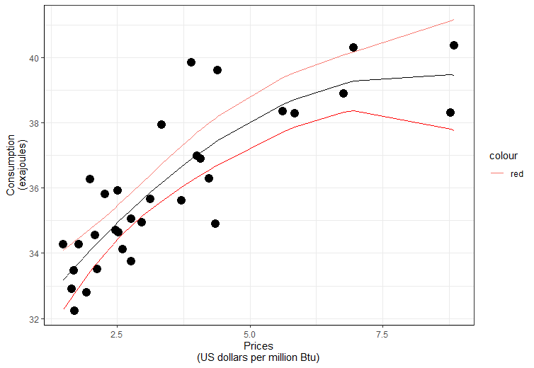
Figure 3. Confidence limits for the regression function.
Measures of the prediction errors
The accuracy of regression analysis is often measured by prediction errors. The most widely used of these are MAE (mean absolute error), RMSE (root mean square error).
RMSE is similar to a standard deviation because the errors are squared and then it should be taken the square root. RMSE measures in the same units as the predicted variable.
The MAE is similar to the RMSE, except that absolute values of errors are used instead of squared errors.
It is possible to choose the best degree of the fitted polynomial model by minimizing MAE, RMSE. However, small values of these measures guarantee only that the model takes into account the historical observations. There is still no guarantee that the model will predict accurately.
Hence, the calculation of measures of the prediction errors can be easily performed using library(Metrics):
library(Metrics)
RMSE<- rmse(data$Consumption, data$fit)
RMSE
[1] 1.195792
MAE<-mae(data$Consumption, data$fit)
MAE
[1] 0.9474194
Normal Distribution of Residuals
Random deviations of obtained residuals should have a normal density distribution. First, we need to receive the residuals with the following code:
res<-data.frame(residuals(PolynomMod))
head(res)

Table3
| No of observation | Residuals.PolynomMod | |||
| 1 | -1.3359156 | |||
| 2 | -0.5581323 | |||
| 3 | 1.0856985 | |||
| 4 | 0.5519787 | |||
| 5 | -0.8147299 | |||
| 6 | -1.1831134 |
The first six residuals are represented in Table 3. Then we need to check the normality of the distribution. It is very useful to create density plots of obtained residuals for checking the assumptions and for assessing the goodness of the fit. Hence, we can use the library (ggplot2) for creating a plot of the density distribution of obtained residuals versus normal scores:
ggplot(res, aes(x=residuals.PolynomMod.)) +
  geom_histogram(aes(y=..density..),colour="black",fill=c("white"))+
  geom_density(aes(x=residuals.PolynomMod.,y=..density..),col="blue")+
  stat_function(fun = dnorm, args = list(mean = mean(res$residuals.PolynomMod.), sd = sd(res$residuals.PolynomMod.)),col="red")+
  ylab("Density") + xlab("Residuals")
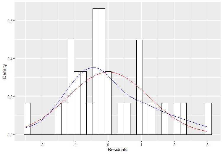
The normal scores in our case are what we would expect to obtain if we take a sample of size n with mean and standard deviation from the residuals represented in Table 3. If the residuals are normally distributed, the picture of obtained residuals should be approximately the same as the normal scores. As we saw from Fig.4. we have a skewed distribution of our residuals and need more checks for this problem.
Another way to check the normality distribution of studentized residuals is the automatic construction of a Quantile-Quantile plot. This plot can be easily constructed with library (car):
library(car)
qqPlot(PolynomMod, labels=row.names(data),simulate=TRUE, main='Q-Q Plot')
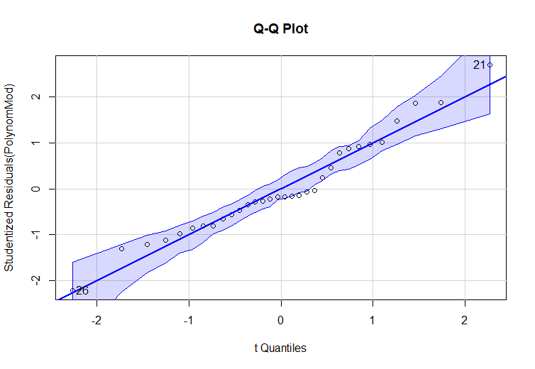
Figure 5. Quantile –Quantile plot of Standardized residuals
On Fig.5 we have a plot of the quantiles of standardized residuals versus the quantiles of normal scores. Here again, if the residuals are normally distributed, the points of standardized residuals should be approximately the same as the points of normal scores. Under normality assumption, this plot should represent a straight line with an intercept of zero (mean) and a slope of the size of the standard deviation of the standardized residuals, i.e. 1. In our case, in Fig.5 we see like in Fig.4 that we have some deviation from the normal distribution. In addition, in Fig.5 we detected the outliers – observations number 21 and 26.
A more complete way of investigation of this problem suggests construction of the plot of the obtained model (7) with the following code:
par(mfrow=c(2,2))
plot(PolynomMod)
As the output of such a code, we obtain 4 diagnostic plots of the regression line, which are shown in Fig. 6. These are:
- Plot of the residuals versus fitted values;
- Normal Quantile-Quantile plot;
- Plot of the standardized residuals versus fitted values;
- Plot of the standardized residuals versus leverage.
The first three plots help to investigate the mentioned above problem with random deviations of the residuals that should have a normal density distribution. The fourth plot also helps to detect influential points and outliers.
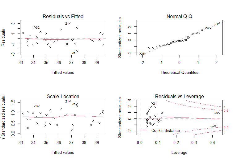
Figure 6. Diagnostic plots of the regression line.
Influential points and outliers
When we fit a model, we should be sure that the choice of the model is not determined by one or a few observations.
Such observations are called influential points and outliers. A point is an influential point if its deletion causes significant changes in the fitted model. Otherwise, observations with large standardized residuals are called outliers because they lie far from the fitted regression line. Since the standardized residuals are approximately normally distributed with mean zero and a standard deviation which is equal to 1, points with standardized residuals larger than 2 or 3 standard deviations away from the 0 are called outliers.
Cook’s distance measures the difference between the regression coefficients obtained from the full statistical data and the regression coefficients obtained by deleting the ith observation. As we see from Fig.6, points number 20 and 17 are influential points, points number 21 and 26 are outliers.
Furthermore, we can create the plot, which shows it more clearly with the following code:
library(car)
influencePlot(PolynomMod, id=TRUE)
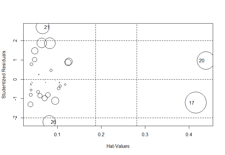
Figure 7. Influence plot.
In Fig.7. we can see the influence plot which shows the most influential points and outliers. The size of the circles is proportional to the degree of influence of observation. Thus the most influential observations are 20 and 17. Two observations 21 and 26 layout from the intervals of Studentized residuals [-2;2]. They are outliers.
Random deviations
The Durbin-Watson (DW) test is the basic test of autocorrelation in regression analysis. The test is based on the assumption that successive residuals are correlated, namely,

In equitation (9) ρ is the correlation coefficient between et and et-1 and wt is normally independently distributed with zero mean and constant variance. Therefore, the residuals have first-order autoregressive structure or first-order autocorrelation.
In most situations, the residuals et may have a much more complex correlation structure. The first-order dependency structure, given in (9), is taken as a simple approximation to the actual error structure. The Durbin-Watson test can be simply calculated by using library (cars):
durbinWatsonTest(PolynomMod)
lag Autocorrelation D-W Statistic p-value
  1       0.4133839      1.030031   0.002
Alternative hypothesis: rho != 0
In our case, the criteria of DW test is equal to 0.4133839, p-value – 0.002 with a significance level of 0.05. Hence, we conclude that the value of DW criteria is significant at the 5% level and Ho is rejected, showing that autocorrelation is present.
The model must be linear with respect to its parameters
Such a hypothesis we can test using function crPlots from the library (cars):
crPlots(PolynomMod)
The output of the abovementioned code is creating Component plus Residual Plot, which is shown in Fig.8. The residual plus component plot for Xm is a scatter plot of (ei+β*mXm) versus Xm where ei is the ordinary least squares residuals when Y is regressed on all predictor variables and β*m is the coefficient of Xm in this regression. β*mXm is the component of the m-th predictor to the fitted values. This plot indicates whether any nonlinearity is present in the relationship between Y and Xm. The plot can therefore suggest possible transformations for linearizing the data. The indication of nonlinearity is, however, not present in the added-variable plot because the horizontal scale in the plot is not the variable itself. Both plots are useful, but the residual plus component plot is more sensitive than the added-variable plot in detecting nonlinearities in the variable being considered for introduction in the model. In our case, we do not indicate nonlinearity.
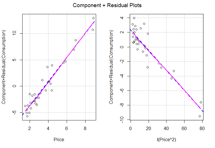
Figure 8. Component plus Residual plot
The variance of random deviations should be constant

When the variance of the residual is not constant over all the observations, the residuals is named heteroscedastic. Heteroscedasticity is usually detected by suitable graphs of the residuals such as the scatter plot of the standardized residuals against the fitted values or against each of the predictor variables.
The most common numeric test for detecting heteroscedasticity is the Breush-Pagan test, which is fulfilled in library (cars):
ncvTest(PolynomMod)
Non-constant Variance Score Test
Variance formula: ~ fitted.values
Chisquare = 0.2052648, Df = 1, p = 0.6505
This test creates a statistic that is chi-squared distributed and for our data equals 0.2052648. The p-value is the result of the chi-squared test and) the null hypothesis is accepted for p-value > 0.05. In this case, the null hypothesis of homoscedasticity would be accepted. Thus, the test result is significant (p = 0.6505), which indicates the fulfillment of the condition of dispersion homogeneity
Data Transformation and Eliminating Outliers
Hence, autocorrelation and homoscedasticity are presented in our model. In this case, we need to overcome such requirements. The most popular way for this is to transform one or more variables (for example, use log (Y) instead of Y) in our model. To help this task, we can use spreadLevelPlot from the library (cars):
spreadLevelPlot(PolynomMod)
Suggested power transformation:  0.2792151
The suggested power transformation is the power of p (Yp), raising to which removes the variance in the residuals. The proposed power transformation is 0.279151, which is close to 0. Thus, we need to use the logarithmic transformation Y in the regression equation, which could give a model that satisfies the abovementioned requirement.
As a result, we make the ln(Y) transformation. Instead of working with Y, we work with ln(Y), a variable, which has an approximate variance
var(log(data$Consumption))
[1] 0.003927263
Consequently, model (7) transforms in:

Then we also can eliminate detected outliers. After transformation our data with following code, we will take the new data, represented in Table 3 for fitting a regression line.
data<-data[-c(21,26),]
data$Consumption<-log(data$Consumption)
head(data)
Table 4
| Year | Natural Gas: Consumption (Exajoules) | Price (US dollars per million Btu) | ||
| 1989 | 3.473212 | 1.696667 | ||
| 1990 | 3.49383 | 1.638333 | ||
| 1991 | 3.534422 | 1.486667 | ||
| 1992 | 3.534069 | 1.771667 | ||
| 1993 | 3.511691 | 2.120833 | ||
| 1994 | 3.490143 | 1.920000 |
Polynomial Regression Model comparison with ANOVA
Therefore, we can obtain our new model (10) and the summary information with the following code:
NEWMod1 <- lm(Consumption ~ Price+I(Price^2), data=data)
summary(NEWMod1)
Call:
lm(formula = Consumption ~ Price + I(Price^2), data = data)
Residuals:
      Min        1Q    Median        3Q       Max
-0.044090 -0.021613 -0.004892  0.021458  0.063086
Coefficients:
             Estimate Std. Error t value             Pr(>|t|)
(Intercept)  3.415397   0.025459 134.152 < 0.0000000000000002 ***
Price        0.064589   0.012771   5.057            0.0000261 ***
I(Price^2)  -0.003983   0.001279  -3.113              0.00434 **
---
Signif. codes:  0 ‘***’ 0.001 ‘**’ 0.01 ‘*’ 0.05 ‘.’ 0.1 ‘ ’ 1
Residual standard error: 0.02964 on 27 degrees of freedom
Multiple R-squared:  0.7918,    Adjusted R-squared:  0.7763
F-statistic: 51.33 on 2 and 27 DF,  p-value: 0.0000000006319
We can increase the degree of the polynom with the next model:
NEWMod2 <- lm(Consumption ~ Price+I(Price^2)+I(Price^3), data=data)
The two nested models can be compared in terms of fit to the data using the anova function. In our case, the nested model is a model, all of which are members of another model.
anova(NEWMod1, NEWMod2)
Analysis of Variance Table
Model 1: Consumption ~ Price + I(Price^2)
Model 2: Consumption ~ Price + I(Price^2) + I(Price^3)
  Res.Df      RSS        Df  Sum of Sq      F     Pr(>F)
1     27     0.023717
2     26     0.023630  1 0.00008701 0.0957    0.7595
From the output of the ANOVA table, we can see the value of the residual sum of squares (RSS) also known as the sum of squared errors (SSE), and the F value. The difference between models 1 and 2 is the degree of the polynomial. In our case, model 1 is embedded in model 2. Since the test result is insignificant (p = 0.7595), we conclude that increasing the degree of the polynomial does not improve the quality of the model, so a polynomial model of degree 2 is sufficient.
Cross-validation for Polynomial Regression Model
Another method to make the existing model better is a method of cross-validation. In cross-validation, part of the data is used as a training sample, and part as a test sample. The regression equation is fitted to the training set and then applied to the test set. Since the test sample is not used to fit the model parameters, the applicability of the model to this sample is a good estimate of the applicability of the obtained model parameters to new data.
In k-fold cross-validation, the sample is divided into k subsamples. Each of them plays the role of a test sample, and the combined data of the remaining k – 1 subsample is used as a training group. The applicability of k equations to k test samples is fixed and then averaged.
Method of cross-validation can be implemented with the library (caret) and the following code:
library(caret)
To perform 10-fold cross-validation:
Preprocess<- trainControl(method = "cv", number = 5)
#fit a regression model and use k-fold CV to evaluate performance
NEWMod3 <- train(Consumption ~ Price+I(Price^2), data = data, method = "lm", trControl = Preprocess)
> summary(NEWMod3$finalModel)
Call:
lm(formula = .outcome ~ ., data = dat)
Residuals:
      Min        1Q    Median        3Q       Max
-0.044090 -0.021613 -0.004892  0.021458  0.063086
Coefficients:
              Estimate Std. Error t value             Pr(>|t|)
(Intercept)   3.415397   0.025459 134.152 < 0.0000000000000002 ***
Price         0.064589   0.012771   5.057            0.0000261 ***
`I(Price^2)` -0.003983   0.001279  -3.113              0.00434 **
---
Signif. codes:  0 ‘***’ 0.001 ‘**’ 0.01 ‘*’ 0.05 ‘.’ 0.1 ‘ ’ 1
Residual standard error: 0.02964 on 27 degrees of freedom
Multiple R-squared:  0.7918,    Adjusted R-squared:  0.7763
F-statistic: 51.33 on 2 and 27 DF,  p-value: 0.0000000006319
As we can see, from the last listing, the use of the transformed data and method of cross-validation allowed to improve the quality of our model from R2=0.7 to R2=0.7763.
Conclusion
The exact determination of the regression equation is the most important product of the regression analysis. It is a summary of the relationship between the response variable and the predictor or set of predictor variables. The obtained equation may be used for several purposes. It may be used to evaluate the importance of individual variables, to analyze the effects of the predictor variables, or to predict values of the response variable for a given set of predictors
As we have seen regression, analysis consists of a set of data analytic techniques that are used to help understand the interrelationships among variables in a certain environment. The task of regression analysis is to learn as much as possible about the environment reflected by the data. We emphasize that what is uncovered along the way to the formulation of the equation may often be as valuable and informative as the final equation.
The media shown in this article is not owned by Analytics Vidhya and are used at the Author’s discretion


