A Quick Tutorial on Clustering for Data Science Professionals

This is article was published as a part of the Data Science Blogathon.

Welcome to this wide-ranging article on clustering in data science! There’s a lot to unpack so let’s dive straight in.

In this article, we will be discussing what is clustering, why is clustering required, various applications of clustering, a brief about the K Means algorithm, and finally in detail practical implementations of some of the applications using clustering.

Table of Contents

1. What is Clustering?
2. Why is Clustering required?
3. Various applications of Clustering
4. A brief about the K-Means Clustering Algorithm
5. Practical implementation of Popular Clustering Applications

What is Clustering?

In simple terms, the agenda is to group similar items together into clusters, just like this:

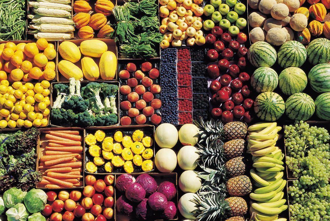
Let’s go ahead and understand this with an example, suppose you are on a trip with your friends all of you decided to hike in the mountains, there you came across a beautiful butterfly which you have never seen before. Further, you encountered a few more. They are not exactly the same but similar enough for you to understand that they belong to the same species. Now here you need a lepidopterist(the one who studies and collects butterflies) to tell you exactly what species they are, but there is no need for an expert to identify a similar group of items. This way of identifying similar objects/ items is known as clustering.

Why is Clustering required?

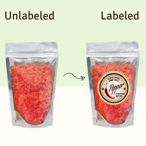
So Clustering is an unsupervised task. Unsupervised means the ones in which we are not provided with any assigned labels or scores for training our data.

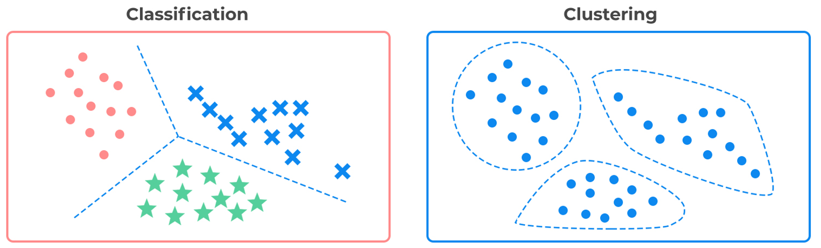
Here in the above figure on the left, we can see that each instance is marked with different markers which means it’s a labeled dataset for which we can use the classification algorithms like SVM, Logistics Regression, Decision Trees, or Random Forests. On the right side if you observe it is the same dataset but without labels so here the story for classifications algorithms ends(i.e we can’t use them here). This is where the clustering algorithms come into the picture to save the day!. Right now in the above picture, it is pretty obvious and quite easy to identify the three clusters with our eyes, but that we not be the case while working with real and complex datasets.

Various applications of Clustering

1. Search engines:

You may be familiar with the concept of image search which Google provides. So what this system does is that first, it applies the clustering algorithm on all the images available in the database available. After which similar images would fall under the same cluster. So when a particular user provides an image for reference what it will be doing is applying the trained clustering model on the image to identify its cluster once this is done it simply returns all the images from this cluster.

2. Customer Segmentation:

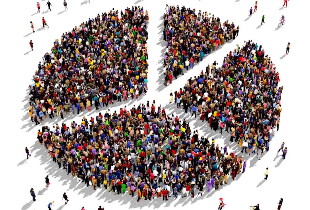
We can also cluster our customers based on their purchase history and their activity on our website. This is really important and useful to understand who our customers are and what they require so that our system can adapt to their requirements and suggest products to each respective segment accordingly.

3. Semi-supervised Learning:

When you are working on semi-supervised learning in which you are only provided with a few labels, there you could perform clustering algorithms and generate labels for all instances falling under the same cluster. This technique is really good for increasing the number of labels after which a supervised learning algorithm can be used and its performance gets better.

4. Anomaly detection:

Any instance that has a low affinity(Measure of how well an instance fits into a particular cluster) is probably an anomaly. For example, if you have clustered the user based on the request per minute on your website,  you can detect users with abnormal behavior. So this technique is particularly useful in detecting any manufacturing detects or for some fraud detections.

5. Image Segmentation:

If you cluster all the pixels according to their colors, then after that we can replace each pixel with the mean color of its cluster, this might be helpful whenever we need to reduce the number of different colors in the image. Image segmentation plays an important part in object detection and tracking systems.

We will look at how to implement this further.

A Brief About the K-Means Clustering Algorithm

Let’s go ahead and take a quick look at what the K-means algorithm really is.

Firstly, let’s generate some blobs for a better understanding of the unlabelled dataset.

import numpy as np
from sklearn.datasets import make_blobs

blob_centers = np.array(
    [[ 0.2,  2.3],
     [-1.5 ,  2.3],
     [-2.8,  1.8],
     [-2.8,  2.8],
     [-2.8,  1.3]])
blob_std = np.array([0.4, 0.3, 0.1, 0.1, 0.1])

X, y = make_blobs(n_samples=2000, centers=blob_centers,
                  cluster_std=blob_std, random_state=7)

Now let’s plot them

plt.figure(figsize=(8, 4))
plt.scatter(X[:, 0], X[:, 1], c=None, s=1)
save_fig("blobs_plot")
plt.show()

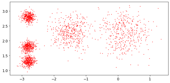
So this is how an unlabeled dataset would look like, here we can clearly see that there are five blobs of instances. So basically k means is just a simple algorithm capable of clustering this kind of dataset efficiently and quickly.

Let’s go ahead and train a K-Means on this dataset. Now, this algorithm will try to find each blob’s center.

from sklearn.cluster import KMeans

k = 5
kmeans = KMeans(n_clusters=k, random_state=101)
y_pred = kmeans.fit_predict(X)

Keep in mind that we need to specify the number of cluster k that the algorithm needs to find. In our example, it is pretty straight forward but in general, it won’t be that easy. Now after training each instance would have been assigned to one of the five clusters. Remember that here an instance’s label is the index of the cluster, don’t confuse it with class labels in classification. 

Let’s take a look at the five centroids the algorithm found:

kmeans.cluster_centers_

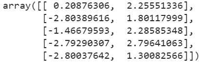
These are the centroids for clusters with indexes of 0,1,2,3,4 respectively.

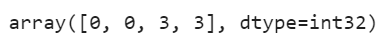
Now you can easily be able to assign new instances and the model will assign it to a cluster whose centroid is closet to it.

new = np.array([[0, 2], [3, 2], [-3, 3], [-3, 2.5]])
kmeans.predict(new)

 

That is pretty much it for now, we will see in detail working and types of K-Means some other day in some other blog. Stay Tuned!

 

Implementation of Popular Clustering Applications

1. Image Segmentation using clustering

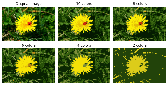
Image Segmentation is just the task of partitioning an image into multiple segments. For example, in a self-driving car’s object detection system, all the pixels that are part of a traffic signal’s image might be assigned to the “traffic-signal” segment. Today there are state of the art model based on CNN(convolution neural network) using complex architecture are being used for image processing. But we are going to do something much simpler which is color segmentation. We will simply assign pixels to a particular cluster if they have the same color. This technique might be sufficient for some applications, like the analysis of satellite images to measure the forest area coverage in a region, color segmentation might just do the work.

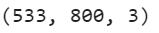
Let’s go ahead a load the image we are about to work on:

from matplotlib.image import imread
image = imread('lady_bug.png')
image.shape

Now Let’s go ahead and reshape the array to get a long list of RGB colors and then cluster them using K-Means:

X = image.reshape(-1, 3)
kmeans = KMeans(n_clusters=8, random_state=101).fit(X)
segmented_img = kmeans.cluster_centers_[kmeans.labels_]
segmented_img = segmented_img.reshape(image.shape)

Now what’s happening here is, for example, it tries to identify a color cluster for all shades of green. After that, for each color, it looks for the mean color of the pixel’s color cluster. What I mean is it will replace all shades of green with a light green color assuming that the mean is light green. At last, it will reshape this long list of colors to the original dimension of the image.

Output with a different number of clusters:

2. Data preprocessing using Clustering

For Dimensionality reduction clustering might be an effective approach, like a preprocessing step before a supervised learning algorithm is implemented. Let’s take a look at how we can reduce the dimensionality of the famous MNIST dataset using clustering and how much performance difference we get after doing this.

MNIST dataset consists of 1797 grayscale(one channel) 8 X 8 images representing digits from 0 to 9. Let’s start by loading the dataset:

from sklearn.datasets import load_digits
X_digits, y_digits = load_digits(return_X_y=True)

Now let’s split them into training and test set:

from sklearn.model_selection import train_test_split
X_train, X_test, y_train, y_test = train_test_split(X_digits, y_digits, random_state=42)

Now let’s go ahead and train a logistic regression model and evaluate its performance on the test set:

from sklearn.linear_model import LogisticRegression
log_reg = LogisticRegression()
log_reg.fit(X_train, y_train)

Now Let’s evaluate its accuracy on the test set:

log_reg_score = log_reg.score(X_test, y_test)
log_reg_score

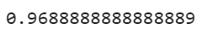
Ok so now we have an accuracy of 96.88%. Let’s see if we can do better by using K-Means as a preprocessing step. We will be creating a pipeline that will first cluster the training set into 50 clusters and replace those images with their distances to these 50 clusters, then after that, we will apply the Logistic Regression model:

Let’s evaluate this pipeline on test set:

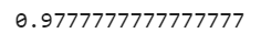
Boom! We just increased the accuracy of the model. But here we choose the number of clusters k arbitrarily. Let’s go ahead and apply grid search to find a better k value:

param_grid = dict(kmeans__n_clusters=range(2, 100))
grid_clf = GridSearchCV(pipeline, param_grid, cv=3, verbose=2)
grid_clf.fit(X_train, y_train)

Warning the above step might be time-consuming!

Let’s see the best cluster that we got and its accuracy:

grid_clf.best_params_

The accuracy now is:

grid_clf.score(X_test, y_test)

Here we got a significant boost in accuracy compared to earlier on the test set.

End Notes

To sum up, in this article we saw what is clustering?, why is clustering required? , various applications of clustering, a brief about the K Means algorithm, and lastly in detail practical implementations of some of the applications using clustering. I hope you liked it!

Karan