Application of Tree-Based Models for Healthcare analysis – Breast Cancer Analysis

This article was published as a part of the Data Science Blogathon

Overview

Decision trees for healthcare analysis are the most widely used machine learning algorithms used for both classification and regression tasks. These are powerful algorithms that can fit complex data. These algorithms form the basis of ensemble algorithms in machine learning. In this article, our focus will be on understanding the core concepts of the Decision Tree for healthcare analysis, followed by understanding the different ensemble techniques. We will then cover Random Forest; an excellent machine learning algorithm developed using decision trees.

Scope of the project

The use case aims to provide hands-on application and understanding of:

1) Data Preprocessing and Exploratory Data Analysis for the data set.

2) Train Tree-Based Models and experiment with hyper-parameters.

3) Apply the trained model for testing data and making predictions.

Problem description in Decision Tree

Breast cancer is the most prevalent cancer in women in cities, and the second most common cancer in women in rural areas. We identify most breast cancers at an advanced stage is because of a lack of knowledge of the disease and the lack of a breast cancer screening program.

This causes the development of innovative methods for detecting breast cancer at an early stage. We hope to show the possibilities of a Decision tree for healthcare analysis-based machine learning algorithms in the early detection of breast cancer through test results and features in this case study.

Because we are categorizing whether the tissue is cancerous or benign, we will train multiple Tree-based models for this procedure. We’ll experiment with hyper-parameters to see if we can enhance the accuracy. Try to solve the problem using the approach outlined below. For further information on each feature, consult the data dictionary.

How to perform Split?

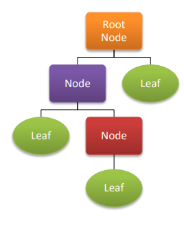
 Branching in decision trees for healthcare analysis aims to make the resultant nodes as pure as possible, i.e., they should contain similar data points. Purity denotes the homogeneity of the instances in the nodes. The most frequently used purity functions are entropy and Gini-index criterion.

 • Entropy: It is the measure of impurity and randomness in the dataset. Let us suppose you chose a girl from a class of 30 girls. The probability of selecting a girl from this class is, therefore, 1. Then this class is said to have no impurity or total purity. Now let’s assume 10 boys were admitted to the above class. Now the probability of choosing a boy from the above class has gone down to 0.75. This denotes that impurity in the dataset has increased while purity has decreased.

Information gain is another metric for splitting that uses entropy as an impurity measure to split the node such that it gives the maximum amount of information gain.

  • Gini-Index: It denotes the probability of a particular instance being wrongly classified when chosen randomly. Gini-index is calculated by subtracting the sum of squared probabilities of each class from one.

We made the split such that it results in the least amount of impurity. The range of the Gini index is between 0 and 1. If all the elements belong to a particular class, the Gini index is 0, while 1 denotes random distribution. We know that decision trees used the divide-and-conquer strategy to divide the datasets into homogenous sets based on purity functions.

 Let us see how we can train a decision tree model in Python.

Step 1: Loading the dataset from sklearn datasets and understanding the data:

from sklearn.datasets import load_breast_cancer
X,y = load_breast_cancer(return_X_y=True, as_frame=True)
print(X.dtypes)
print()

Output:

 

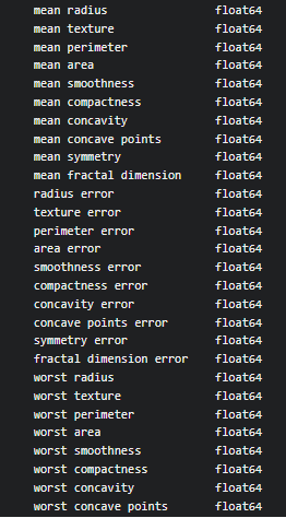
Go through dtypes attribute to check data types of all columns of X.

Step 2: Check for missing Values/Null Values and display a count plot for the target variable.

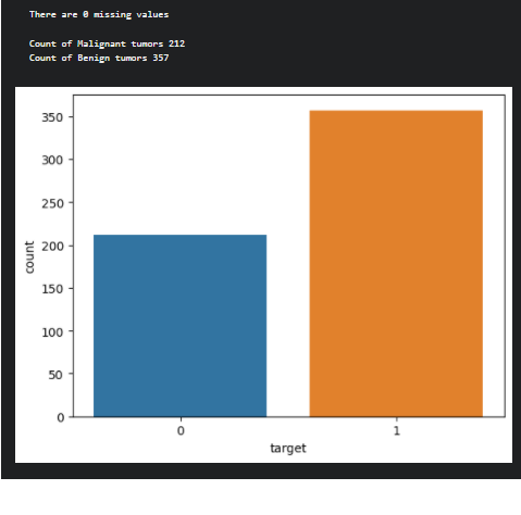
isnull function used to check the missing values in the data set. Use the value_counts function on the target variable to check the count of each category in the target column and plot it using a count plot.

print(f'There are {pd.concat([X,y], axis=1).isnull().sum().sum()} missing values')
print()
print(f'Count of Malignant tumors {y.value_counts()[0]}')
print(f'Count of Benign tumors {y.value_counts()[1]}')
ax = sns.countplot(y, label='Count')  
plt.show()

Output

After analyzing the data, next prepare the data for preprocessing.

Data Preparation in Decision Tree

Data preparation aims to prepare the data for the machine learning model. We will remove correlated features and split the dataset for training and testing to build a tree-based model.

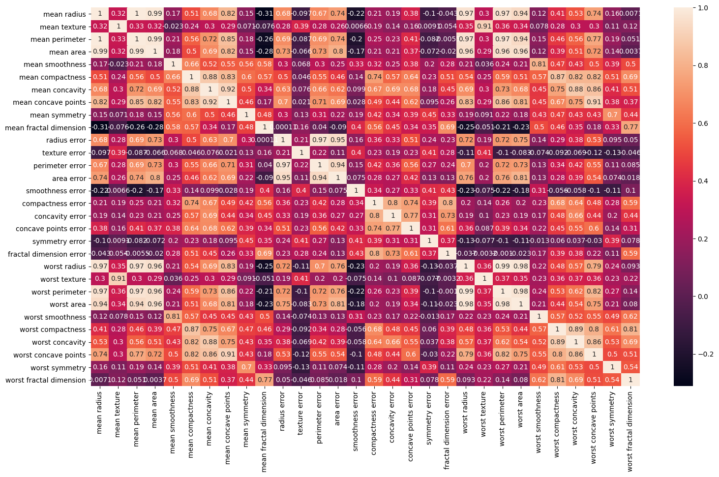
Step 3: We can use a heatmap to visualize the correlation values

Use the heatmap method to display correlation values from the corr() function of the pandas data frame.

plt.figure(figsize=(18,10))
sns.heatmap(X.corr(), annot=True)
plt.show()

Output

Step 4

Remove highly correlated values

Use the drop method to drop the highly correlated features. The reason behind it is when there are two highly correlated independent variables, delete one of them since you’ll run into the multicollinearity problem, and the regression coefficients for the two highly linked variables in your regression model will be unreliable.

Storage and performance considerations have also driven the removal of highly correlated variables. Aside from that, the only thing that counts concerning features is if they help with prediction and whether the data quality is enough.

drop_list = ['mean perimeter','mean radius','mean compactness','mean concave points','radius error','perimeter error','compactness error','concave points error','worst radius','worst perimeter','worst compactness','worst concave points','worst texture','worst area']
X = X.drop(drop_list, axis=1)

Step 5: Next step is to split the data into train and test data:

We use the train_test_split class from sklearn.model_selection module to split the dataset into the train and test with the following attributes.

from sklearn.model_selection import train_test_split
X_train, X_test, y_train, y_test = train_test_split(X, y, test_size = 0.2, random_state = 42)

After performing the data split, check the shape of training and test data:
shape attribute is used to check the shape of the datasets.

print(f'The shape of Train data is {X_train.shape}')
print(f'The shape of Test data is {X_test.shape}')

Output:

Implementation of Decision Tree Algorithm

Source: sklearn.tree.DecisionTreeClassifier

For classification and regression, Decision Trees (DTs) for healthcare analysis are a non-parametric supervised learning method. The goal is to learn simple decision rules from data attributes to develop a model that predicts the value of a target variable. A tree is an approximation of a piecewise constant.

Decision trees use a series of if-then-else decision rules to estimate a sine curve using data. The decision criteria become more complex as the tree grows deeper and the model becomes more accurate.

It aims at fitting the “Decision Tree algorithm” on the training dataset and evaluating the performance of the model for the testing dataset.

Step 6

At first, we have to create an instance of the algorithm

Use DecisionTreeClassifier class from sklearn.tree package to create an instance of the Decision Tree algorithm. Use criterion as “gini” and a maximum depth of 2.

from sklearn.tree import DecisionTreeClassifier
tree_clf = DecisionTreeClassifier(criterion='gini', max_depth=2)

Next, we need to fit the algorithm on the training dataset,

Use the fit() method to fit the algorithm on the training data.

tree_clf.fit(X_train, y_train)

To make predictions on the test data, we use predict method to make predictions on the test data.

y_test_pred = tree_clf.predict(X_test)

It’s time to calculate the accuracy and confusion matrix of the model,

To calculate the accuracy and confusion matrix of the model, we have to use accuracy_score and confusion_matrix metrics to evaluate the performance of the model.

from sklearn.metrics import confusion_matrix, accuracy_score
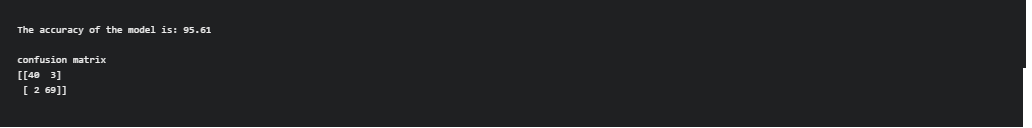
print(f'The accuracy of the model is: {accuracy_score(y_test,y_test_pred)*100:0.2f}')
print()
print('confusion matrix')
print(f'{confusion_matrix(y_test, y_test_pred)}')

Output:

Random Forest Classifier

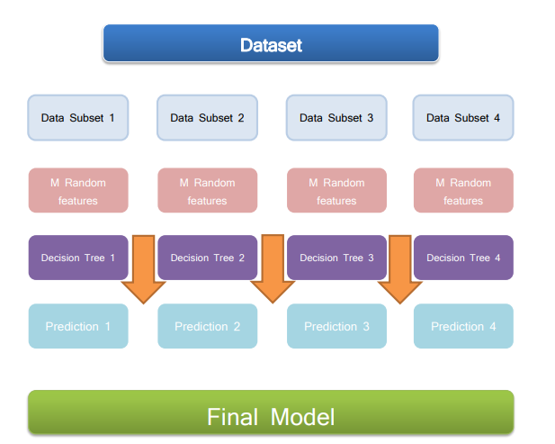
A random forest is a meta estimator that employs averaging to increase predicted accuracy and control over-fitting by fitting several decision tree classifiers for healthcare analysis on various sub-samples of the dataset. If bootstrap=True (default), the max sample argument regulates the sub-sample size; otherwise, the entire dataset is used to create each tree.

The random forest comprises three parts from a broader perspective. These are:

Random Forest = Decision Trees + Bagging + Feature sampling

Step7: After fitting the model on the training data, the next step is to make predictions and test the performance of the model that has been built.

To create an instance of the algorithm, Use RandomForestClassifier class from sklearn.ensemble package to create an instance of the algorithm. Use n_estimators as 100 and the random state as 32.

from sklearn.ensemble import RandomForestClassifier
rf_clf = RandomForestClassifier(n_estimators=100, random_state=32)

Next comes fitting the algorithm on the training dataset. We have to use the fit method to fit the algorithm on the training data with two parameters, i.e., X_train and y_train.

rf_clf.fit(X_train, y_train)

Let’s now make the predictions on the test data with a random forest classifier.

y_train_pred = rf_clf.predict(X_train)
y_test_pred = rf_clf.predict(X_test)

Finally, calculate the accuracy and confusion matrix of the model. For that, we have to use accuracy_score and confusion_matrix metrics to evaluate the performance of the model.

print(f'The accuracy of the model on the train data: {accuracy_score(y_train, y_train_pred)*100:0.2f}')
print(f'The accuracy of the model on the test data: {accuracy_score(y_test, y_test_pred)*100:0.2f}')
print()
print('confusion matrix')
print(f'{confusion_matrix(y_test, y_test_pred)}')

Output

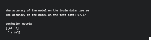
Here, the accuracy of the training data is 100, This happens when the model memorizes the noise and fits too close to the training set. The model becomes “overfitted,”. Here, the model is overfitted and we need an optimization algorithm to fit the model.

Hyper parameter-tuned Random Forest Classifier

Hyper-parameter

Selecting a set of ideal hyper-parameters for a learning algorithm is known as hyperparameter optimization or tuning. A hyper-parameter is a value for a parameter that is used to influence the learning process. Other factors, such as node weights, are learned.

We can tune the performance of the model using various parameters that can fix it before fitting the model on the training data. In this step, we will see different parameters associated with random forest algorithms that can help to control the performance of the model.

Step 8

Tuning the features of the Random Forest Classifier.

Use RandomForestClassifier class from sklearn.ensemble package to create an instance of the algorithm. We will reduce the number of decision trees used to build the model (using n_estimators = 10) and fit the depth of the decision tree (max_depth) to 5. Also, use n_jobs = -1 to use all cores for training.

rf_clf = RandomForestClassifier(n_estimators=10, max_depth=5, random_state=32, n_jobs=-1)
rf_clf.fit(X_train, y_train)
y_train_pred = rf_clf.predict(X_train)
y_test_pred = rf_clf.predict(X_test)

Finally, calculate the accuracy and confusion matrix of the Hyper-parameter tuned model. we need to use accuracy_score and confusion_matrix metrics to evaluate the performance of the model.

print(f'The accuracy of the model on the train data: {accuracy_score(y_train, y_train_pred)*100:0.2f}')
print(f'The accuracy of the model on the test data: {accuracy_score(y_test, y_test_pred)*100:0.2f}')
print()
print('confusion matrix')
print(f'{confusion_matrix(y_test, y_test_pred)}')

Output

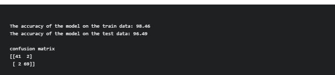
By evaluating the performance of the Hyper-parameter tuned model, the hyper-parameter tuner outputs the setting that yields the highest performing model. The final stage is to build a new model using the best hyper-parameter settings on the complete dataset (training and validation). As a result, the accuracy of train data is 98.46% and test data is 96.49 per cent, respectively, on the hyper-parameter tuning.

Summary

Key takeaways for the decision tree in healthcare analysis are as follow:

1) Tree-Based models are essential tools for any data science professional journey since it is intuitive to explain the tree-based models. In contrast, other machine learning models function as a black box.

2) we started with an introduction to Decision Trees and explained the algorithms’ working. We studied the metrics used for splitting a node. Then we implemented the algorithm on a regression problem through Python.

I hope this blog will be more informative and interesting!

If you have questions, please leave them in the comments area. In the meantime, check out my other articles here!

Know About the Author

Hello, my name is Lavanya, and I’m from Chennai. I am a passionate writer and enthusiastic content maker. The most intractable problems always thrill me. I am currently pursuing my B. Tech in Computer Science Engineering and have a strong interest in the fields of data engineering, machine learning, data science, and artificial intelligence, and I am constantly looking for ways to integrate these fields with other disciplines such as science and chemistry to further my research goals.

Linkedin Profile: https://www.linkedin.com/in/lavanya-srinivas-949b5a16a/

Thank you for reading!

The media shown in this article is not owned by Analytics Vidhya and are used at the Author’s discretion.