Evaluating A Classification Model for Data Science

This article was published as a part of the Data Science Blogathon.

Introduction to Evaluation of Classification Model 

As the topic suggests we are going to study Classification model evaluation. Before starting out directly with classification let’s talk about ML tasks in general.
Machine Learning tasks are mainly divided into three types

1. Supervised Learning — In Supervised learning, the model is first trained using a Training set(it contains input-expected output pairs). This trained model can be later used to predict output for any unknown input.
2. Unsupervised Learning — In unsupervised learning, the model by itself tries to identify patterns in the training set.
3. Reinforcement Learning —  This is an altogether different type. Better not to talk about it.

Supervised learning task mainly consists of Regression & Classification. In Regression, the model predicts continuous variables whereas the model predicts class labels in Classification.

For this entire article, let’s assume you’re a Machine Learning Engineer working at Google. You are ordered to evaluate a handwritten alphabet recognizer. Train classifier model, training & test set are provided to you.

The first evaluation metric anyone would use is the “Accuracy” metric. Accuracy is the ratio of correct prediction count by total predictions made. But wait a minute . . .

Is Accuracy enough to evaluate a model?

Short answer: No

So why is accuracy not enough? you may ask

Before answering this, let’s talk more about classification.
For simplicity purposes, we assume a classifier which outputs whether the input alphabet is “A” or not.
So there are four distinct possibilities as shown below

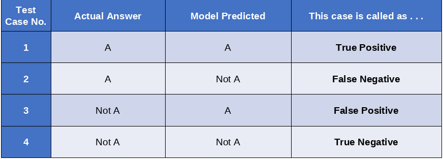
The above table is self-explanatory. But just for the sake of some revision let’s briefly discuss it.

1. If the model predicts “A” as an “A”, then the case is called True Positive.
2. If the model predicts “A” a “Not A”, then the case is called False Negative.
3. If the model predicts “Not A” as an “A”, then the case is called False Positive.
4. If the model predicts “Not A” as a “Not A”, then the case is called True Negative

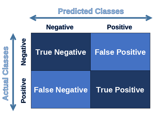
Another easy way of remembering this is by referring to the below diagram.

As some of you may have already noticed, the Accuracy metric does not represent any information about False Positive, False Negative, etc. So there is substantial information loss as these may help us evaluate & upgrade our model.

Okay, so what are other useful evaluation metrics?

Confusion Matrix for Evaluation of Classification Model

A confusion matrix is a n x n matrix (where n is the number of labels) used to describe the performance of a classification model. Each row in the confusion matrix represents an actual class whereas each column represents a predicted class.

Confusion Matrix can be generated easily using confusion_matrix() function from sklearn library.
The function takes 2 required parameters
1) Correct Target labels
2) Predicted Target labels

## dummy example
from sklearn.metrics import confusion_matrix
y_true = ["cat", "ant", "cat", "cat", "ant", "bird"]
y_pred = ["ant", "ant", "cat", "cat", "ant", "cat"]
confusion_matrix(y_true, y_pred, labels=["ant", "bird", "cat"])
>>> array([[2, 0, 0],
[0, 0, 1],

           [1, 0, 2]])

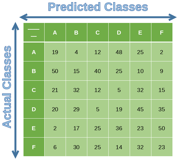
We will take a tiny section of the confusion matrix above for a better understanding.

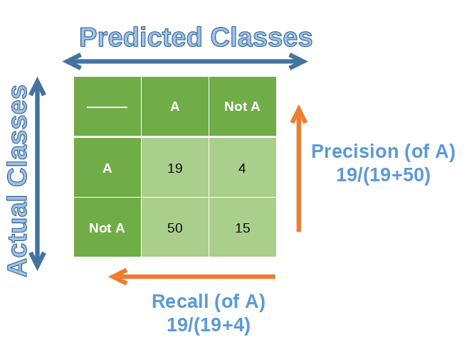
Precision

Precision is defined as the ratio of True Positives count to total True Positive count made by the model.
Precision =  TP/(TP+FP)

Precision can be generated easily using precision_score() function from sklearn library.
The function takes 2 required parameters
1) Correct Target labels
2) Predicted Target labels

## dummy example
from sklearn.metrics import precision_score
y_true = [0, 1, 1, 0, 1, 0]
y_pred = [0, 0, 1, 0, 0, 1]
precision_score(y_true, y_pred)
>>> 0.5

Precision in itself will not be enough as a model can make just one correct positive prediction & return the rest as negative. So the precision will be 1/(1+0)=1. We need to use precision along with another metric called “Recall”.

Recall

Recall is defined as the ratio of True Positives count to the total Actual Positive count.
Recall = TP/(TP+FN)
Recall is also called “True Positive Rate” or “sensitivity”.

Recall can be generated easily using recall_score() function from sklearn library.
The function takes 2 required parameters
1) Correct Target labels
2) Predicted Target labels

## dummy example
from sklearn.metrics import recall_score
y_true = [0, 1, 1, 0, 1, 0]
y_pred = [0, 0, 1, 0, 0, 1]
recall_score(y_true, y_pred)
>>> 0.333333

Hybrid of both

There is another classification metric that is a combination of both Recall & Precision. It is called the F1 score. It is the harmonic mean of recall & precision. The harmonic mean is more sensitive to low values, so the F1 will be high only when both precision & recall are high.

Recall can be generated easily using f1_score() function from sklearn library.
The function takes 2 required parameters
1) Correct Target labels
2) Predicted Target labels

## dummy example
from sklearn.metrics import f1_score
y_true = [[0, 0, 0], [1, 1, 1], [0, 1, 1]]
y_pred = [[0, 0, 0], [1, 1, 1], [1, 1, 0]]
f1_score(y_true, y_pred, average=None)
>>> array([0.66666667, 1. , 0.66666667])

Ideal Recall or Precision

We can play with the classification model threshold to adjust recall or precision. In reality, there is no ideal recall or precision. It all depends on what kind of classification task is it. For example, in the case of a cancer detection system, you’ll prefer having high recall & low precision. Whereas in the case of an abusive word detector, you’ll prefer having high precision but low recall.

Precision/Recall Trade-off

Sadly, increasing recall will decrease precision & vice versa. This is called Precision/Recall Trade-off.

Precision & Recall vs Threshold

We can plot precision & recall vs threshold to get information about how their value changes according to the threshold. Here below is a dummy graph example.

## dummy example

from sklearn.metrics import precision_recall_curve

precisions, recalls, thresholds = precision_recall_curve(y_true, y_predicted)

plt.plot(thresholds, precisions[:-1], "b--", label="Precision")

plt.plot(thresholds, recalls[:-1], "g-", label="Recall")
plt.show()

As you can see as the threshold increases precision increases but at the cost of recall. From this graph, one can pick a suitable threshold as per their requirements.

Precision vs Recall

Another way to represent the Precision/Recall trade-off is to plot precision against recall directly. This can help you to pick a sweet spot for your model.

ROC Curve for Evaluation of Classification Model 

ROC stands for Receiver Operating Characteristics. It is a graph of True Positive Rate (TPR) vs False Positive Rate(FPR).
1. TPR means recall.
2. FPR is the ratio of Negative classes inaccurately being classified as positive.

TPR=TP/(TP+FN)
FPR = FP/(FP+TN)

Below is a dummy code for ROC curve.

from sklearn.metrics import roc_curve
fpr, tpr, thresholds = roc_curve(y_true, y_predicted)
plt.plot(fpr, tpr, linewidth=2, label=label)
plt.plot([0, 1], [0, 1], 'k--') 
plt.show()

In the below example graph, we have compared ROC curves for SGD & Random Forest Classifiers.

ROC curve is mainly used to evaluate and compare multiple learning models. As in the graph above, SGD & random forest models are compared. A perfect classifier will transit through the top-left corner. Any good classifier should be as far as possible from the straight line passing through (0,0) & (1,1). In the above graph, you can observe that the Random Forest model is working better compared to SGD.  PR curve is preferred over ROC curve when either the positive class is rare or you prioritize more about False Positive.

Conclusion

So that’s it for now. We studied classification model evaluation & talked about multiple evaluation metrics.

Sources

All Graphs are provided on : https://www.divakar-verma.com/post/h-o-m-l-chapter-3-classification

The media shown in this article is not owned by Analytics Vidhya and are used at the Author’s discretion