This article was published as a part of the Data Science Blogathon

Introduction

In today’s digital world, social media platforms like Facebook, Whatsapp, Twitter have become a part of our everyday schedule. Many NLP techniques can be used on the text data available from Twitter. Sentiment analysis refers to the idea of predicting the sentiment ( happy, sad, neutral) from a particular text. In this blog, I will be performing sentiment analysis on a large real-world dataset by applying techniques of NLP(Natural Language Processing).

I am taking my data from the “Sentiment140” dataset available in Kaggle. It has around 1.6 million tweets that have been extracted. You can access the dataset here: dataset. The annotations or labels for the tweets are as follows:

• 0 = negative

• 4 = positive

Data for Sentiment Analysis

Let us start by importing libraries and reading the data from csv files.

import pandas as pd
df = pd.read_csv('../input/sentiment140/training.csv',header=None)
df.head(8)

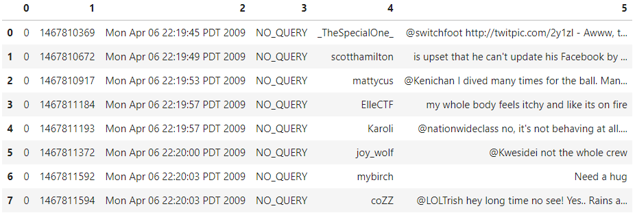
                                                                                             Source: Kaggle notebook of Author

The first column is the target column, which will denote the sentiment of the tweets (0/2/4). The next column is the ID for each tweet, and it is a unique number. After that, we have the date and timestamp of when the tweet was released. Next, we have the username of the author of the tweet. In the end, we have the text of the tweet. You can notice that the columns and renamed accordingly.

df.columns = [‘sentiment’, ‘id’, ‘date’, ‘query’, ‘user_name’, ‘tweet’]

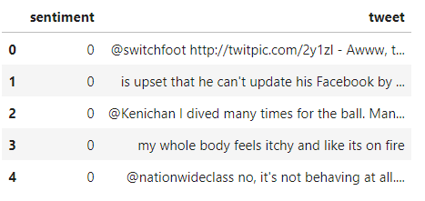
In this blog, the focus is on classifying the sentiment of the text. Hence, we can drop the unnecessary columns as shown below.

df = df.drop(['id', 'date', 'query', 'user_name'], axis=1)
df.head()

Let us map the sentiment values to positive, negative. 0 is mapped to negative, and four is mapped to positive. We create a small function `mapper()` to perform this mapping. This function can be used on all the dataset rows using the “apply()” function.  Look at the code snippet below.

label_to_sentiment = {0:"Negative", 4:"Positive"}
def mapper(label):
     return label_to_sentiment[label]
df.sentiment = df.sentiment.apply(lambda x: label_decoder(x))

Class balance is an important criterion when we are working on classification problems. It is essential to ensure that the classes are not very skewed, and the class imbalance will lead to biased results. Let us look at the distribution.

distribution = df.sentiment.value_counts()
plt.figure(figsize=(8,4))
plt.bar(distribution.index, distribution.values)

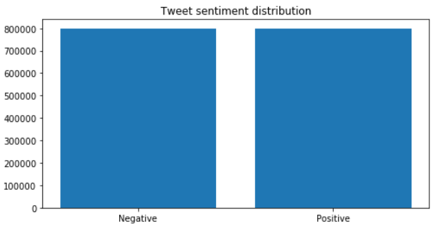
 Source: Kaggle notebook of Author

Lucky for us, the data is not skewed much. Let’s move to an essential part of any NLP task: Text pre-processing.

Text for Sentiment Analysis Pre-processing

There is a lot of noise in the raw text data scrapped from the tweets. The two critical parts of text cleaning for sentiment analysis include: stop word removal and stemming.

There are punctuations, symbols that will not contribute to our model much. There are also stop words present which need to be removed. Stop words refer to the connecting words like ‘the,’ ‘and’ ‘was,’ which do not provide any specific meaning, which will not help our analysis. Hence, we remove these and clean the data.  NLTK is a python package used commonly for NLP tasks. Using this package, we can quickly get all the stopwords in English. Have a look at the below snippet.

# Import nltk package and download the stopwords
import nltk 
nltk.download('stopwords')
# We filter out the english language stopwrds
from nltk.corpus import stopwords
stop_words = stopwords.words('english')
print(stop_words)

Stemming/lemmatization refers to the process of extracting the root word. For example, can write ‘play’ as ‘playing,’ ‘played,’ ‘plays’ in different tenses. But the actual meaning is the same. We need to convert these into the root word for easier modelling. We can use the Snowball stemmer from the NLTK package to implement this. This is a rectified version of Porter’s stemmer algorithm.

from nltk.stem import SnowballStemmer

stemmer = SnowballStemmer('english')

For removing the non-alphabetic characters, we can use regex expressions.

import re
text_cleaning_regex = "@S+|https?:S+|http?:S|[^A-Za-z0-9]+"

Now, let us define a function that will perform regex filtering, stop word removal, and stemming on all the tweets. Note that in NLP,  we describe the processed words as ‘tokens.’ Each tweet will be passed on to the function shown below.

def clean_tweets(text, stem=False):
  # Text passed to the regex equatio
  text = re.sub(text_cleaning_regex, ' ', str(text).lower()).strip()
  # Empty list created to store final tokens
  tokens = []
  for token in text.split():
    # check if the token is a stop word or not
    if token not in stop_words:
      if stem:
        # Paased to the snowball stemmer
        tokens.append(stemmer.stem(token))
      else:
        # A
        tokens.append(token)
  return " ".join(tokens)

What’s happening in this function?

The text is converted into all lower case; white spaces are stripped and passed to the equation. The hyperlinks will remove non-alphanumeric characters. An empty list can be created to store the final tokens. The sentence is split into words, and each word is checked if it belongs to the list of stop words or not. After that, stemming is performed, and the word is stored in the list.  In the end, the tokens in the list are joined and returned.

df.tweet = df.tweet.apply(lambda x: clean_tweets(x))

Lets us move on to the modelling part next.

First, let us split the dataset into train and test sets. We can do this easily using the `train_test_split()` function of the sklearn library. We take 20% of the dataset for testing purposes and the rest for training.

# Import functions from sklearn library
from sklearn.model_selection import train_test_split
from sklearn.preprocessing import LabelEncoder
# Splitting the data into training and testing sets
train_data, test_data = train_test_split(df, test_size=0.2,random_state=16)
print("Train Data size:", len(train_data))
print("Test Data size", len(test_data))
#> Train Data size: 1280000
#> Test Data size 320000

Tokenization & Label Encoding

Tokenization refers to splitting the given sentence into a list of tokens, indexed or vectorized.  We will be using TensorFlow and Keras for modelling. Keras has a pre-processing module for text, which offers us the `tf.keras. pre-processing.text.Tokenizer()` class. You can initialize it as shown below. You can also specify the splitting criteria, the maximum number of words, and so on.

from keras.preprocessing.text import Tokenizer
tokenizer = Tokenizer()

This class has `fit_on_texts()` method. If we pass a list of texts to this function, we will update the internal vocabulary accordingly.

tokenizer.fit_on_texts(train_data.tweet)
word_index = tokenizer.word_index
print(word_index)

This is a dictionary where each word is mapped with a particular index, starting from 1.

vocab_size = len(tokenizer.word_index) + 1
print("Vocabulary Size :", vocab_size)
#> Vocabulary Size : 290415

We will be applying a sequence model to this data. For this, we need to pass inputs of the same size. To achieve this, we will use the `pad_sequences()` function. This will return us sequences of a constant size, which can be passed as a parameter. Take a look at the code snippet. We have set the sequence length as 30 in this case.

from keras.preprocessing.sequence import pad_sequences
# The tokens are converted into sequences and then passed to the pad_sequences() function
x_train = pad_sequences(tokenizer.texts_to_sequences(train_data.tweet),maxlen = 30)
x_test = pad_sequences(tokenizer.texts_to_sequences(test_data.tweet),maxlen = 30)

Next, let us move on to label encoding. The sklearn library’s pre-processing module provides us with a Label encoder class. Initialize and fit it upon the training dataset’s labels (sentiment column). After this, we extract the sentiment from train data to make y_test, y_train by encoding and reshaping, as shown below.

labels = ['Negative', 'Positive']
from sklearn.preprocessing import LabelEncoder
encoder = LabelEncoder()
encoder.fit(train_data.sentiment.to_list())
y_train = encoder.transform(train_data.sentiment.to_list())
y_test = encoder.transform(test_data.sentiment.to_list())
y_train = y_train.reshape(-1,1)
y_test = y_test.reshape(-1,1)

Now, we have successfully split them into dependent and independent sets.

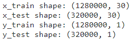
Source: Kaggle notebook of Author ( Shapes of training and testing sets)

GloVe Word Embeddings

Word embeddings are used to represent words with vectors. The ultimate aim is that the talks with similar meanings are closer to each other than the irrelevant words in the vector representation. The distance between the words could be measured by cosine similarity. For example, the words’ travelling’ and ‘vacation’ will be represented by vectors closer to each other.

The gloVe is a pretrained word embedding model, and we can download it.

!wget http://nlp.stanford.edu/data/glove.6B.zip
!unzip glove.6B.zip

Now, we can create a dictionary mapping the words with GloVe vector representations.

embeddings_index = {}
# opening the downloaded glove embeddings file
f = open('/kaggle/working/glove.6B.300d.txt')
for line in f:
    # For each line file, the words are split and stored in a list
    values = line.split()
    word = value = values[0]
    coefs = np.asarray(values[1:], dtype='float32')
    embeddings_index[word] = coefs
f.close()
print('Found %s word vectors.' %len(embeddings_index))

#> Found 400000 word vectors

Recall that in the tokenizing section, we had gotten a dictionary ‘word_index’, where each word is mapped to an index in the vocabulary. Now, we will map those vocab indices with the glove representations.

# creating an matrix with zeroes of shape vocab x embedding dimension
embedding_matrix = np.zeros((vocab_size, 300))
# Iterate through word, index in the dictionary
for word, i in word_index.items():
    # extract the corresponding vector for the vocab indice of same word
    embedding_vector = embeddings_index.get(word)
    if embedding_vector is not None:
        # Storing it in a matrix
        embedding_matrix[i] = embedding_vector

Now, we have a matrix that can initialize the weights. We will be using the embedding layer of Keras.

embedding_layer = tf.keras.layers.Embedding(vocab_size,300,weights=[embedding_matrix],
                                          input_length=30,trainable=False)

Model architecture – LSTM

LSTM stands for Long Short Term Memory. It is a modified and advanced architecture of the RNNs ( Recurrent Neural Networks). It is mainly helpful in sequential problems of NLP, where RNN fails due to vanishing and exploding gradients. LSTMs are capable of long-range modelling dependencies with better accuracy than conventional networks.

If you are new to Deep learning, you might want to check out this article for a deeper understanding of how LSTM works.

In this problem, our architecture consists of four main parts. We start with the embedding layer defined previously, and it inputs the sequences and gives word embeddings. These embeddings are then passed on to the convolution layer, which will convert them into small feature vectors. Next, we have the bidirectional LSTM layer. After the LSTM layers, we have a couple of Dense (fully connected layers) for classification purposes. We use a sigmoid activation function before the final output.

# Import various layers needed for the architecture from keras
from tensorflow.keras.layers import Conv1D, Bidirectional, LSTM, Dense, Input, Dropout
from tensorflow.keras.layers import SpatialDropout1D
from tensorflow.keras.callbacks import ModelCheckpoint
# The Input layer 
sequence_input = Input(shape=(30,), dtype='int32')
# Inputs passed to the embedding layer
embedding_sequences = embedding_layer(sequence_input)
# dropout and conv layer 
x = SpatialDropout1D(0.2)(embedding_sequences)
x = Conv1D(64, 5, activation='relu')(x)
# Passed on to the LSTM layer
x = Bidirectional(LSTM(64, dropout=0.2, recurrent_dropout=0.2))(x)
x = Dense(512, activation='relu')(x)
x = Dropout(0.5)(x)
x = Dense(512, activation='relu')(x)
# Passed on to activation layer to get final output
outputs = Dense(1, activation='sigmoid')(x)
model = tf.keras.Model(sequence_input, outputs)

Model Training and Results

The model architecture is complete. Let us move on to train the model on the dataset. We will use the Adam optimizer. Since its a binary classification task ( positive or negative sentiment), we can use the Binary Cross-Entropy loss function.

Generally, it is helpful to alter the learning rate during the training for minor dataset training problems. For this, we can use the Learning rate Schedulers. The ReduceLROnPLateau will decrease the learning rate by a factor of 0.1 (can be specified) if the validation loss is not falling. Here, the monitor used in ReduceOnPlateau is the validation loss. AUC could also be used instead.

from tensorflow.keras.optimizers import Adam
from tensorflow.keras.callbacks import ReduceLROnPlateau
model.compile(optimizer=Adam(learning_rate=LR), loss='binary_crossentropy',metrics=['accuracy'])
ReduceLROnPlateau = ReduceLROnPlateau(factor=0.1,min_lr = 0.01, monitor = 'val_loss',verbose = 1)

You should decide the batch size and the number of epochs you will train for. In general, training for 10-20 epochs is sufficient.

training = model.fit(x_train, y_train, batch_size=1024, epochs=10,
                    validation_data=(x_test, y_test), callbacks=[ReduceLROnPlateau])

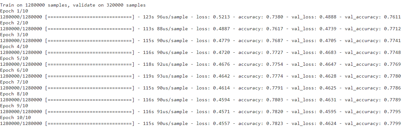
Source: Training console of Author

Evaluation of the Sentiment Analysis Model

I plotted the training and validation accuracy against the epochs. The validation accuracy is around 0.78, as we can see in the below image.

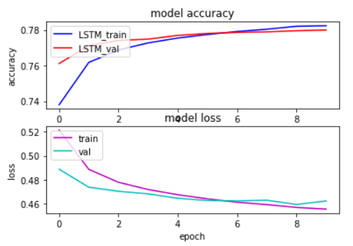
                                                                                                    Source: Training console of Author

Now that the model is trained, we can make predictions with it. In the end, this is a binary classification case. So, it would help to choose a threshold value to classify the data samples.  I am choosing 0.5, and if the prediction is above 0.5, then the tweet is classified as positive. Otherwise, it is classified as negative.

def predict_tweet_sentiment(score):
    return "Positive" if score>0.5 else "Negative"
scores = model.predict(x_test, verbose=1, batch_size=10000)
model_predictions = [predict_tweet_sentiment(score) for score in scores]

Now, let us compare the forecasts against the actual test data values.

from sklearn.metrics import classification_report
print(classification_report(list(test_data.sentiment), model_predictions))

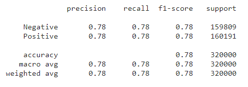
         Source: Author’s Kaggle Notebook

From the above image, we can observe that the precision is around 0.78. These values are good enough.

I hope you liked my article on Sentiment Analysis!

Connect with me: [email protected]

The media shown in this article is not owned by Analytics Vidhya and are used at the Author’s discretion.