Time Series Forecasting with Extreme Learning Machines

 This article was published as a part of the dataset

Introduction

Making predictions about the future from historical data available (time series forecasting) is a very important tool with a wide variety of applications like product demand forecasting, weather, and climate forecasting, forecasting in the healthcare sector, etc. There are two main approaches to time series forecasting – statistical approaches and neural network models. The most popular statistical method for time series forecasting is the ARIMA (Autoregressive Integrated Moving Average) family with AR, MA, ARMA, ARIMA, ARIMAX, and SARIMAX methods. In this article, however, we are going to discuss a neural network approach to time series forecasting using extreme learning machines.

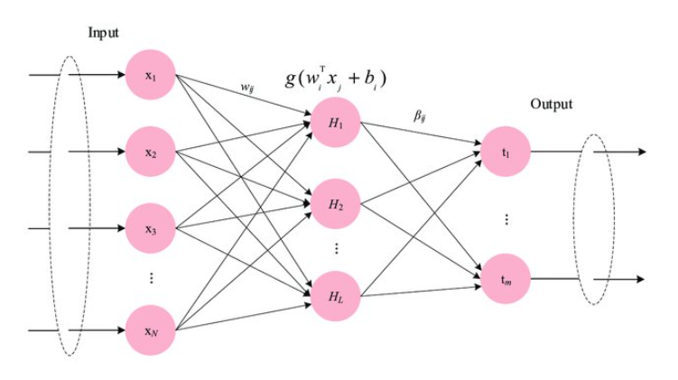
Extreme learning machines are single hidden layer feedforward neural networks proposed by Huang et. al. in 2004. They have extremely fast learning speed, good generalization performance, and universal approximation capabilities. The weights and the biases of the hidden layer nodes are set randomly, thus saving time required in hyper tuning by backpropagation. The weights of the output layer can be determined analytically by a Moore Penrose inverse operation.

How do ELMs work?

The ELM algorithm can be described as follows :

1. The weights and the biases of the hidden layer are randomly assigned.
2. The hidden layer output matrix (H) is calculated by multiplying the inputs with the randomly assigned weights, adding biases, and finally applying an activation function on the output.
3. The output weight matrix is calculated by multiplying the Moore Penrose inverse of H (hidden layer output matrix) with the training data matrix (T).
4. The output weight matrix is finally used to make predictions on new data.

A pictorial depiction of an extreme learning machine is given below :

Why use ELMs?

The main advantage of extreme learning machines is that they take much less training time compared to traditional back-propagated neural networks. In traditional feedforward neural network models, the weights and the biases of the hidden layers are tuned iteratively with slow gradient-based learning algorithms like backpropagation. Since the hidden layer weights and the biases are randomly assigned in ELMs, they are computationally much faster than traditional deep neural network models. In addition to their computational efficiency, ELMs have been shown to be more advantageous in terms of efficiency and generalization performance over traditional FNN algorithms on a wide range of benchmark problems from different fields (Refer to Paper 1, Paper 2 for further details). ELMs have also been shown to have universal approximation capabilities (Refer to Paper 3).

Time series forecasting – ELMs vs traditional methods 

In the context of time series forecasting, ELMs can be a really powerful tool. Statistical approaches to times series modeling like ARIMA models can only be applied to stationary time series (whose properties do not depend on the time at which the series is observed), they fail to capture seasonality. Neural network models can overcome this difficulty as they help in capturing the non-linearity in data due to external factors. Traditional backpropagated NNs however suffer from certain drawbacks like overfitting, slow learning speed, etc. ELMs are better than backpropagated NNs as they have extremely fast learning speed, good generalization performance, and least human intervention.

Overcoming the disadvantages

The main disadvantage of ELMs is that the stochasticity involved in the algorithm might sometimes lead to sub-optimal performance in terms of accuracy. To overcome this, one must properly tune the hyperparameters involved like the number of hidden nodes, the type of activation function, etc. This tuning is sometimes done using metaheuristic optimization algorithms like Bayesian Optimisation, Genetic Algorithms, Teaching-Learning Based Optimisation algorithm, etc. A number of variants of ELM have also come out which overcome these drawbacks like the optimally pruned ELM, online sequential ELM, etc. but their discussion is outside the purview of this blog.

Since their inception, ELMs have been used in a wide variety of fields like object recognition, feature learning, clustering, classification, regression, and time-series modeling with promising results. Now that we know what ELMs are and how they work, let us dive right into trying to perform time series forecasting with them.

Loading the Time Series Dataset 

We are going to be using a product demand dataset from a gaming console store. The dataset has daily sales data of a product from January 2013 to December 2017. Data from January 2013 to September 2017 is used for training and October 2017 to December 2017 data is used for testing.

import pandas as pd
from datetime import datetime
def parser(x):
    return datetime.strptime(x,"%Y-%m-%d")
data = pd.read_csv('Sales_Data.csv', header = 0, parse_dates=[0],index_col=0, date_parser=parser)
print(data.head())

Source: Screenshot from my Jupyter Notebook

We can visualize the time series data using matplotlib :

import matplotlib.pyplot as plt
%matplotlib inline
data = data.astype(float)
data
data.plot(style='k.',ylabel='Sales')
plt.show()

The plotted dataset looks like this :

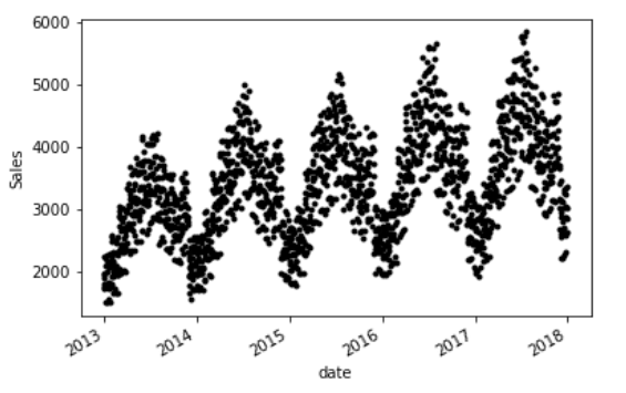
Source: Screenshot from my Jupyter Notebook

We can see that the dataset shows certain clear trends, which makes forecasting easier.

Next, we import certain necessary packages and convert the data to a NumPy array to make operations easier :

from sklearn.metrics import mean_squared_error
import math
import numpy as np
from scipy.linalg import pinv2
data = np.array(data)
data = np.reshape(data, (-1, 1))
data

Making Train-Test Splits and Data Normalisation  

We need to split the data into training and testing parts and perform data normalization.

m = 14
per = (1736 - m)/1826
size = int(len(data) * per)
d_train, d_test = data[0:size], data[size:len(data)]
mean_train = np.mean(d_train)
sd_train = np.std(d_train)
d_train = (d_train-mean_train)/sd_train
d_test = (d_test-mean_train)/sd_train

There are a number of things to note in the above code snippet. We first split the data into training and testing parts. We will try to forecast the last 3 months of daily sales and use the rest of the data for training. For predicting the daily sales data at any time step, we need to provide values of previous time steps data as input (which is known as the lag). Here, we have chosen the lag size as 14, i.e. sales data of the previous 14 days is used to predict the next day’s sales data. m here represents the lag size. We have accordingly performed the train-test split.

Data normalization is an essential preprocessing task to be performed in any forecasting job. In this code, the time series data has been normalized by subtracting the mean and then dividing by the standard deviation of data. The predictions will need to be transformed back to the original scale using the corresponding denormalization equation.

Next, we need to reshape the train and test data into the form that needs to be fed into the ELM.

X_train = np.array([d_train[i][0] for i in range(m)])
y_train = np.array(d_train[m][0])
for i in range(1,(d_train.shape[0]-m)):
    l = np.array([d_train[j][0] for j in range(i,i+m)])
    X_train = np.vstack([X_train,l])
    y_train = np.vstack([y_train,d_train[i+m]])
X_test = np.array([d_test[i][0] for i in range(m)])
y_test = np.array(d_test[m][0])
for i in range(1,(d_test.shape[0]-m)):
    l = np.array([d_test[j][0] for j in range(i,i+m)])
    X_test = np.vstack([X_test,l])
    y_test = np.vstack([y_test,d_test[i+m]])
print(X_train.shape)
print(y_train.shape)
print(X_test.shape)
print(y_test.shape)
#> (1708, 14)
#> (1708, 1)
#> (90, 14)
#> (90, 1)

As mentioned earlier, we are feeding 14 previous time steps data as input to predict the data at the next step. We use simple NumPy operations to reshape our data so that our final train input data is a 1708 X 14 matrix and the final train output data is a 1708 X 1 matrix. Similar operations are performed for the test data.

Building the ELM model

We have already discussed the ELM algorithm earlier. The ELM model has a number of hyperparameters that need to be optimized for optimal performance – lag size, number of hidden nodes, input weights and biases, and the type of activation function.

import scipy.stats as stats
input_size = X_train.shape[1]
hidden_size = 100   #no. of hidden neurons
mu, sigma = 0, 1
w_lo = -1 
w_hi = 1
b_lo = -1 
b_hi = 1
#initialising input weights and biases randomly drawn from a truncated normal distribution
input_weights = stats.truncnorm.rvs((w_lo - mu) / sigma, (w_hi - mu) / sigma, loc=mu, scale=sigma,size=[input_size,hidden_size])
biases = stats.truncnorm.rvs((b_lo - mu) / sigma, (b_hi - mu) / sigma, loc=mu, scale=sigma,size=[hidden_size])
def relu(x):      #hidden layer activation function
    return np.maximum(x, 0, x)

We are choosing the number of neurons in the hidden layer (hidden_size) as 100. The weights and the biases of the hidden layer are randomly drawn from a truncated normal distribution from (-1,1). The relu activation function is used. We have written our own function ‘relu’ for performing relu activation. You can explore using other activation functions and changing the number of hidden nodes to improve accuracy further.

def hidden_nodes(X):
    G = np.dot(X, input_weights)
    G = G + biases
    H = relu(G)
    return H
output_weights = np.dot(pinv2(hidden_nodes(X_train)), y_train)
def predict(X):
    out = hidden_nodes(X)
    out = np.dot(out, output_weights)
    return out
prediction = predict(X_test)

The function ‘hidden_nodes’ calculates the hidden layer output matrix by multiplying the weights with input vectors and adding the biases. Relu activation is also applied to the output. The Moore Penrose inverse of the hidden layer output matrix is calculated using the pinv2 function from scipy.linalg library. The output weights matrix is stored in output_weights. The function ‘predict’ is used to perform predictions on the test data X_test.

Evaluating Time Series Forecasting

It is important to evaluate the quality of forecasts using some sort of performance metric.

correct = 0
total = X_test.shape[0]
y_test = (y_test*sd_train) + mean_train
prediction = (prediction*sd_train) + mean_train
# evaluate forecasts
rmse = math.sqrt(mean_squared_error(y_test, prediction))
print('Test RMSE: %.3f' % rmse)
mape_sum = 0
for i,j in zip(y_test,prediction):
    mape_sum = mape_sum + (abs((i-j)/i))
mape = (mape_sum/total)*100
mpe_sum = 0
for i,j in zip(y_test,prediction):
    mpe_sum = mpe_sum + ((i-j)/i)
mpe = (mpe_sum/total)*100
print('Test MAPE: %.3f' % mape)
print('Test MPE: %.3f' % mpe)

Three performance metrics are used to evaluate the quality of forecasts – root mean squared error (RMSE), mean percentage error (MPE) and mean absolute percentage error (MAPE). Keep in mind that we need to denormalize the data by multiplying with standard deviation and adding the mean before calculating RMSE, MPE, MAPE, etc. The mean_squared_error function from sklearn.metrics library is used to calculate RMSE while MPE and MAPE are directly calculated using their respective formulae. I obtained the test MAPE as 2.767% but your result might vary due to the stochasticity involved in the algorithm.

How does Time Series Forecasting look?  

We have reached the end of the forecasting task and need to see how our predicted forecasts look. We plot the results using matplotlib again.

# plot forecasts against actual outcomes
fig, ax = plt.subplots(figsize = (10,6))
ax.plot(y_test,label = 'Actual')
ax.plot(prediction, color='red',label = 'Predictions')
ax.legend(loc='upper right', frameon=False)
plt.xlabel('Days',fontname="Arial", fontsize=24, style='italic', fontweight='bold')
plt.ylabel('Sales Data',fontname="Arial", fontsize=24, style='italic', fontweight='bold')
plt.title('Forecasting for last 3 months with ELM (100 hidden nodes)',fontname="Arial", fontsize=24, style='italic', fontweight='bold')
plt.xticks([0,20,40,60,80],['2017-10-02','2017-10-22','2017-11-11','2017-12-01','2017-12-21'],fontname="Arial", fontsize = 20, style='italic')
plt.yticks(fontname="Arial", fontsize = 22, style='italic')

The results look like this :

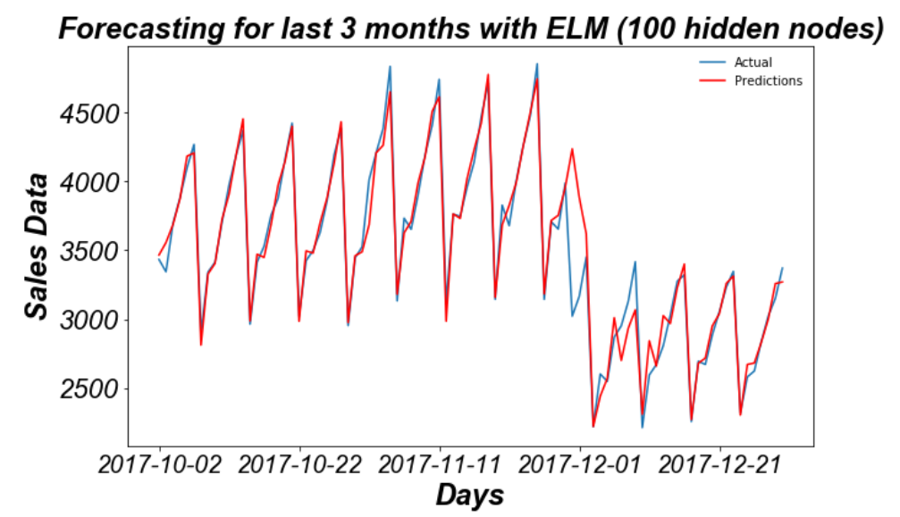
Source: Screenshot from my Jupyter Notebook

Hopefully, by now you understand how extreme learning machines work and how they can be used for time series forecasting. You can explore improving the accuracy further by tuning hyperparameters like the number of hidden nodes, the type of activation function, and the lag size.

Thank you for reading! 🙂

Want to read more about the time series? Head on to our dataset.

Feel free to connect with me over mail: [email protected]

The media shown in this article is not owned by Analytics Vidhya and are used at the Author’s discretion.