Convolutional Neural Network: An Overview

This article was published as a part of the Data Science Blogathon.

Let’s begin the journey!! Let’s start by familiarizing ourselves with the meaning of CNN (Convolutional Neural Network) along with its significance and the concept of convolution.

What is Convolutional Neural Network?

• Convolutional Neural Network is a specialized neural network designed for visual data, such as images & videos. But CNNs also work well for non-image data (especially in NLP & text classification).
• Its concept is similar to that of a vanilla neural network (multilayer perceptron) – It follows the same general principle of forwarding & backward propagation.

Why do we need Convolutional Neural Network?

• Although vanilla neural networks (MLPs) can learn highly complex functions, their architecture does not exploit what we know about how the brain reads & processes images.
• The architecture of Convolutional Neural Network uses many of the working principles of the animal visual system & it has been able to achieve extraordinary results in image-related learning tasks.
• For this reason, MLPs haven’t been able to achieve any significant breakthroughs in the image processing domain.

What is Convolution?

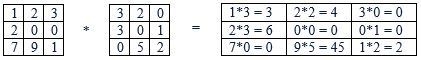
• Mathematically, convolution is the summation of the element-wise product of 2 matrices.
• Let us consider an image ‘X’ & a filter ‘Y’ (More about filter will be covered later). Both of them, i.e. X & Y, are matrices (image X is being expressed in the state of pixels). When we convolve the image ‘X’ using filter ‘Y’, we produce the output in a matrix, say’ Z’.

Source: Author

• Finally, we compute the sum of all the elements in ‘Z’ to get a scalar number, i.e. 3+4+0+6+0+0+0+45+2 = 60

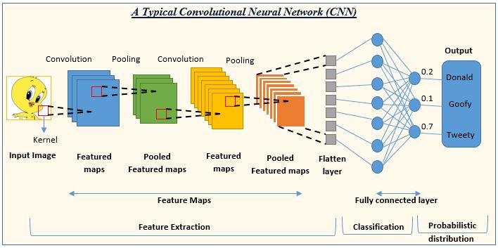
Now that we are familiar with the idea behind CNN let us dig deeper into the topic to understand the building blocks of CNN. Following is the outline of our journey: 

 

What are Filters/Kernels?

• A filter provides a measure for how close a patch or a region of the input resembles a feature. A feature may be any prominent aspect – a vertical edge, a horizontal edge, an arch, a diagonal, etc.
• A filter acts as a single template or pattern, which, when convolved across the input, finds similarities between the stored template & different locations/regions in the input image.
• Let us consider an example of detecting a vertical edge in the input image.
• Each column of the 4×4 output matrix looks at exactly three columns & three rows (the coloured boxes show the output of the filter as it moves over the input image). The values in the output matrix represent the change in the intensity along the horizontal direction w.r.t the columns in the input image.
• The output image has the value 0 in the 1st & last column. It means there is no change in intensity in the first three columns & the previous three columns of the input image. On the other hand, the output is 30 in the 2nd & 3rd column, indicating a change in the intensity of the corresponding columns of the input image.

Dimensions of the Convolved Output?

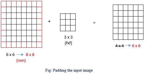
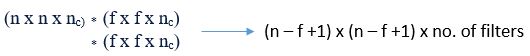
         If the input image size is ‘n x n’ & filter size is ‘f x f ‘, then after convolution, the size of the output image is: (Size of input image – filter size + 1)
x (Size of input image – filter size + 1). Let us refer to the below image:

Source: Author

Why do we do Padding?

•  Every time we apply a convolution operator, our image shrinks (in the above example, our vision shrunk from 6 x 6 to 4 x 4). If we convolve the output again with a filter, our image shrinks.
• If we continue this process, we lose a lot of information because of image shrinking, which is one of the downsides of convolution.
• During convolution, the pixels in the corners & the edges are considered only once. This is the 2nd downside of convolution. If we consider any pixel in the middle, many (fxf) regions overlap the pixel (we shift the filter & observe the image through it, i.e. convolve). Thus, the pixels on the corners or the edges are used much less in the output. So, we throw away a lot of information near the edge of the image.
• So to fix both of these problems, we can ‘pad’ the image.

• Let P be padding. In this example, p = 1 because we padded all around the input image with an extra border of 1 pixel.

⸫ Output Size = (n + 2p –f +1) x (n + 2p –f +1)

                         = (6 + 2×1 – 3 +1) x (6 + 2×1 – 3 +1)

                         = 6 x 6

Let,

n x n = Original input image size

p = Padding

(n+2p) x (n+2p) = Size of padded input image

(n+2p–f+1) x (n+2p-f+1) = Size of output image after convolving padded image

⸫ Output size after convolving padded image = Original input image size

• If the value of ‘f’ is even, we may need asymmetric padding (Please refer above eqn. 1 ). Let us say that the size of the filter i.e. ‘f’ is 6. Then by using equation 1, we get a padding size of 2.5, which does not make sense.

• The 2^nd reason for choosing an odd size filter such as a 3×3 or a 5×5 filter is we get a central position & at times it is nice to have a distinguisher.

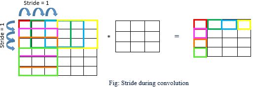
What is Stride?

• The stride indicates the pace by which the filter moves horizontally & vertically over the pixels of the input image during convolution.

Source: Author

• Stride depends on what we expect in our output image. We prefer a smaller stride size if we expect several fine-grained features to reflect in our output. On the other hand, if we are only interested in the macro-level of features, we choose a larger stride size.
• To understand the concept of stride in more detail, let’s consider an example. Let’s say we are interested in classifying the input image between landscape & portrait. We do not need minute details for this task, such as the number of mountain peaks, trees, etc. So we can choose a higher value for stride. On the other hand, if we want to classify an image between dog & cat, we need to focus or capture very minute details or features of the input image to type the image correctly. In this case, we prefer a smaller stride size.

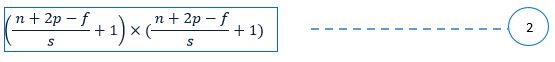
Let,

S = Stride size

⸫ Size of the output image is given by :

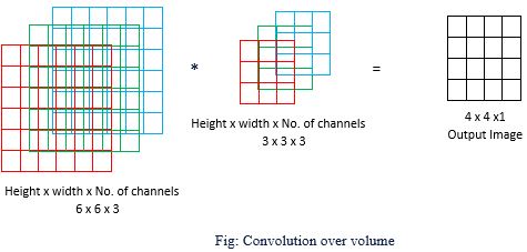
Convolutions over RGB images

• Consider an RGB image of size 6×6. Since it’s an RGB image, its dimension is 6x6x3, where the three corresponds to the three colour channels: Red, Green & Blue. We can imagine this as a 3-D image with a stack of 3 six by six shots.
• For 3-D images, we need 3D filters, i.e. the filter itself will also have three layers corresponding to the red, green & blue channels, similar to that of the input RGB image.

• Convolution operator functions in a similar fashion in both 2D (greyscale) & 3D (RGB) images. We 1^st place the 3x3x3 filter in the upper left most position. This filter has 27 (9 parameters in each channel) or numbers. We take each of these 27 numbers & multiply them with the corresponding numbers from the image’s red, green & blue channels. Then we add up all those numbers & this gives us the 1^st number in the output image.
• To compute the following output, we take this filter & slide/stride it over by 1 (or whatever stride number we consider) & again, due to 27 multiplications, add up the 27 numbers.

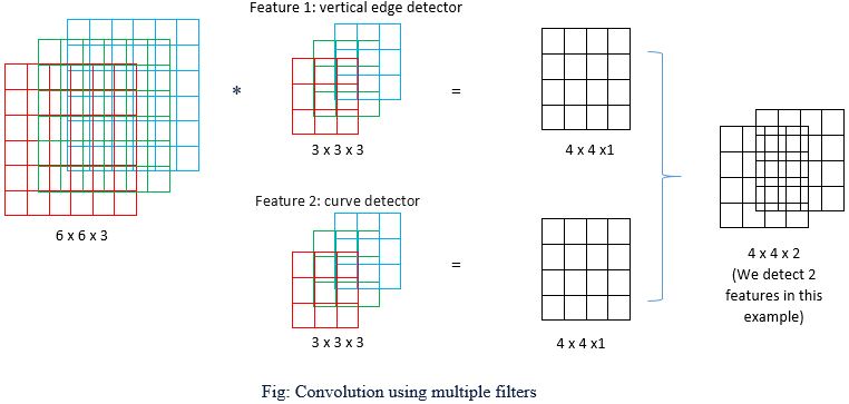
Multiple Filters for Multiple Features

•  We can use multiple filters to detect various features simultaneously. Let us consider the following example in which we see vertical edge & curve in the input RGB image. We will have to use two different filters for this task, and the output image will thus have two feature maps.

Source: Author

• Let us understand the dimensions mathematically,

Some important terms

1. The filters are learned during training (i.e. during backpropagation). Hence, the individual values of the filters are often called the weights of CNN.
2. A neuron is a filter whose weights are learned during training. E.g., a (3,3,3) filter (or neuron) has 27 units. Each neuron looks at a particular region in the output (i.e. its ‘receptive field’)
3. A feature map is a collection of multiple neurons, each looking at different inputs with the same weights. All neurons in a feature map extract the same feature (but from other input regions). It is called a ‘feature map’ because it maps where a particular part is found in the image.

What is Pooling?

• A pooling layer is another essential building block of CNN. It tries to figure out whether a particular region in the image has the feature we are interested in or not.
• The actual dictionary meaning of pooling is the act of sharing or combining two or more things. In CNN, the pooling layer does a similar job. It summarizes the featured map so that the model will not need to be trained on precisely positioned features, making a model more reliable and robust.
• The pooling layer looks at more significant regions (having multiple patches) of the image & captures aggregate statistics (min, max, average & global). In other words, it makes the network invariant to local transformations.
• The two most popular aggregate functions used in pooling are ‘max’ & ‘average’:

1. 1. Max pooling – If any of the patches say something firmly about the presence of a particular feature, then the pooling layer counts that feature as ‘detected’.
   2. Average pooling – If one patch says something very firmly, but the other ones disagree, the average pooling takes the average to find out.

Source: Author

• Pooling has the advantage of making the representation more compact by reducing the spatial size of the feature maps, thereby reducing the number of parameters to be learnt. Pooling reduces only the height & width of the feature map, not the (i.e. number of channels). For example, if we have ‘m’ feature maps each of size (c,c), the pooling operation will produce ‘m’ outputs (c/2,c/2).
• On the other hand, pooling also loses a lot of information, which is often considered a potential disadvantage.
• The pooling layer has ‘NO PARAMETERS’ i.e. ‘ZERO TRAINABLE PARAMETERS’. The pooling layer computes the aggregate of the input. E.g. in max pooling, it takes a maximum over a group of pixels. We do not need any adjustments in any parameters.
• The following image explains when a MAX pooling works and when AVG pooling works:

(Image source: https://www.researchgate.net/publication/300020038_Mixed_Pooling_for_Convolutional_Neural_Networks )

A typical CNN has the following sequence of CNN layers

• We have an input image using multiple filters to create various feature maps.
• Each feature map of size (C, C) is pooled to generate a (C/2, C/2) output (for a standard 2×2 pooling)
• The above pattern is referred to as one Convolutional Neural Network layer or one unit. Multiple such CNN layers are stacked on top of each other to create deep Convolutional Neural Network networks.
• The output of the convolution layer contains features, and these features are fed into a dense neural network.

Read more articles about the convolutional neural network on our blog.

The media shown in this article is not owned by Analytics Vidhya and are used at the Author’s discretion.