Embedding Techniques on Text Data using KNN
This article was published as a part of the Data Science Blogathon.
In this article, we will try to classify Food Reviews using multiple Embedded techniques with the help of one of the simplest classifying machine learning models called the K-Nearest Neighbor.
Here is the agenda that will follow in this article.
- Objective
- Loading Data
- Data Preprocessing
- Text preprocessing
- Time-Based Splitting
- Embedding Techniques
- Types of Embedding Techniques
- BOW
- TF-IDF
- Word2Vec
- Average Word2Vec
- TF-IDF-Word2Vec
- Building Model
- Conclusion
Objective
The objective of this article will be to determine whether a review is positive(3+ rating) or negative (rating 1 or 2). Since the data, we will be working on is text data we will explore different embedding techniques that we can use to reduce high dimensional data to low dimensional data and build models on top of that.
Loading the Data
We will be using Amazon Fine Food Reviews data. It is publicly available on Kaggle.
Data Source: https://www.kaggle.com/snap/amazon-fine-food-reviews
The dataset is available in two forms and we will be using sqlite form to work upon. We are using this form because it is easier to query the data and visualize the data efficiently using SQL.
Since this article’s objective is to determine positive(3+ rating) or negative reviews(3- ratings) we will ignore ratings that are equal to 3 (neutral) while loading the data.
#establishing connection to sqlite database
con=sqlite3.connect('../input/database.sqlite')
#reading the dataset and ignore the neutral reviews
orignal_data=pd.read_sql_query("""SELECT * From Reviews WHERE Score!=3""",con)
Below are the details of the Amazon Fine Food Reviews dataset.
Number of reviews: 568,454
Number of users: 256,059
Number of products: 74,258
Timespan: Oct 1999 – Oct 2012
Number of Attributes/Columns in data: 10
Attribute Information:
- Id
- ProductId – unique identifier for the product
- UserId – unique identifier for the user
- ProfileName
- HelpfulnessNumerator – number of users who found the review helpful
- HelpfulnessDenominator – number of users who indicated whether they found the review helpful or not
- Score – a rating between 1 and 5
- Time – timestamp for the review
- Summary – Brief summary of the review
- Text – Text of the review
Data Preprocessing
Removing Duplicates
Here we are removing such entries that have the same value on ‘UserId’, ‘ProfileName’, ‘Time’, and ‘Text’.
#first sorting according to product id
sort_prodid=orignal_data.sort_values('ProductId',axis=0,inplace=False,kind='quicksort',na_position='last')
data_no_duplicate=sort_prodid.drop_duplicates(subset={"UserId","ProfileName","Time","Text"},keep='first',inplace=False)
data_no_duplicate.shape
HelpfulnessNumerator<=HelpfulnessDenominatior
- HelpfulnessNumerator =Yes (Find Useful)
- HelpfulnessDenominator = Yes+No (Find Useful + Not Find Useful)
- So HelpfulnessNumerator will always be <= HelpfulnessDenominator. Here we are keeping only such entries.
#keeping only the entries where HelpfulnessNumerator<=HelpfulnessDenominator
data_no_duplicate=data_no_duplicate.loc[data_no_duplicate['HelpfulnessNumerator']<=data_no_duplicate['HelpfulnessDenominator']]
Sorting the data on ‘Time’ and keeping only 100k points
My system has 16GB of RAM. I have observed that working on more than 100k data points from the dataset leads to memory overflow in my system. So choose a number of data points as per your system RAM. So, because of Memory Constraints, we will only choose 100K data points.
#sorting the data on the basis of Timestamp
sorted_data_time=data_no_duplicate.sort_values(["Time"],axis=0,ascending=True,inplace=False)
#Selecting 100K points from sorted data
data_100k=sorted_data_time.iloc[0:100000,:]
Converting ‘Score’ to a positive or negative review
#Score attribute ranges between 1 to 5, we have already ignored score 3(neutral).
#So here we are converting score to a positive or negative review
# Score<3 then 0(negative) else 1(positive)
def partition(x):
    if x<3:
        return 0
    else:
        return 1
actual_score=data_100k['Score']
pos_neg_review=actual_score.map(partition)
data_100k['Score']=pos_neg_review
Text Preprocessing
Now we will perform text preprocessing on the ‘Text’ column in the data. this is the column that contains the raw review of the food.
Below are the steps that we will be performing on the ‘Text’ column.
- Removing HTML tags
- Removing Special Characters
- Keeping only the English words
- Converts all words to lowercase
- Remove Stopwords
- Applying Stemming
Now we will write functions that will apply the above-mentioned changes to the ‘Text’ column.
import re
def cleanhtml(sentence):
    cleanr=re.compile('')
    cleansent=re.sub(cleanr,"",sentence)
    return cleansent
def cleanpunc(sentence): #to remove special characters
    cleaned=re.sub(r'[?|!|'|"|#]',r'',sentence)
    cleaned=re.sub(r'[.|,|)|(||/]',r' ',cleaned)
    return cleaned
#below option is not necessary everytime. only if stopword resource is not found then run below command
#nltk.download('stopwords')
import nltk
from nltk.corpus import stopwords
stop=set(stopwords.words('english'))
#initializing the snowball stemmer that will convert the words to their root meaning
sno=nltk.stem.SnowballStemmer('english')
In the above-mentioned text preprocessing steps, steps 1 through 4 are obvious to understand. The last two steps are that need some clarification.
Stopwords are the words that are so commonly used in a language that they carry very little information. Example: ‘a’, ‘the’, ‘is’, ‘are’ etc. While speaking a language they are useful since they carry information about ‘tense’ and also bring together the two different sentences. But while performing NLP or text preprocessing for machine learning models these words do not add much information. For example in this article in a food review model only needs information about a word that represents either positive/negative sentiment and adding any stopword would not change the meaning of that review.
Stemming is a process that converts a word to its root meaning. This is important because in a language words can be written in either tense(present, past, or future) but what we need is the essence of a word so that it can be used to identify positive or negative reviews.
Now, we will apply all the above-mentioned steps to the ‘Text’ and ‘Summary’ columns.
#applying all the steps of preprocessing on Text Attribute
from tqdm import tqdm #to show progress bar
i=0
str1=' '
final_string=[]
s=''
for sent in tqdm(data_100k['Text'].values):
    filtered_sent=[]
    sent=cleanhtml(sent) #cleaning HTML tags
    for w in sent.split():
        for cleaned_words in cleanpunc(w).split():
            if((cleaned_words.isalpha())&(len(cleaned_words)>2)): #keeping only english words
                if(cleaned_words.lower() not in stop):
                    s=(sno.stem(cleaned_words.lower())).encode("utf-8") #stemming
                    filtered_sent.append(s)
                else:
                    continue
            else:
                continue
    str1=b" ".join(filtered_sent)
    final_string.append(str1)
    i+=1
data_100k['CleanedText']=final_string
data_100k['CleanedText']=data_100k['CleanedText'].str.decode("utf-8")
#applying all the steps of preprocessing 'Summary' Attribute
from tqdm import tqdm #for progress baar
i=0
str1=' '
final_string=[]
s=''
for sent in tqdm(data_100k['Summary'].values):
    filtered_sent=[]
    sent=cleanhtml(sent) #cleaning HTML tags
    for w in sent.split():
        for cleaned_words in cleanpunc(w).split():
            if((cleaned_words.isalpha())&(len(cleaned_words)>2)):
                if(cleaned_words.lower() not in stop):
                    s=(sno.stem(cleaned_words.lower())).encode("utf-8")
                    filtered_sent.append(s)
                else:
                    continue
            else:
                continue
    str1=b" ".join(filtered_sent)
    final_string.append(str1)
    i+=1
data_100k['CleanedSummary']=final_string
data_100k['CleanedSummary']=data_100k['CleanedSummary'].str.decode("utf-8")
Now we will drop the original columns and keep the cleaned version on them.
cleantext_data_100k=data_100k.drop(["Text","Summary"],axis=1,inplace=False)
cleantext_data_100k.head()
Time-Based Splitting
Since the reviews provided in the dataset are time-dependent we will be splitting the data using time and not randomly.
We will keep the first 60,000 reviews for training the next 20,000 reviews for cross-validation and the last 20,000 reviews for testing.
#splitting the dataset
train_data=cleantext_data_100k.iloc[0:60000,:]
crossvalidation_data=cleantext_data_100k.iloc[60000:80000,:]
test_data=cleantext_data_100k.iloc[80000:100000,:]
Embedding Techniques
Embedding techniques are used to represent the words used in text data to a vector. Since we can not use text data directly to train a model what we need is representation in numerical form which in turn can be used to train the model. Let’s explore the different embedding techniques.
Types of Embedding Techniques
BOW
BOW means Bag of Words. It is the simplest Embedded technique to represent the text data into a numerical vector. As the name suggests this technique creates a bag of all the words present in the training data. See the below image for a better understanding.
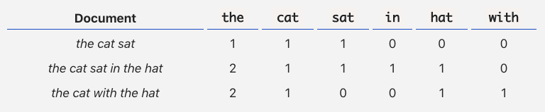
Source: A Simple Explanation of the Bag-of-Words Model | by Victor Zhou | Towards Data Science
The drawback of BOW is that it only counts the occurrence of a word in the sentence and does not take care of the arrangements of the words which in turn loses the relationship of two words present in the sentence if any. Another drawback is that it creates the vector using the training vocabulary of the data and if vocabulary increases several folds then vector size will increase dramatically which can cause memory overflow.
There is one more thing that we can do to retain some sequence information which is to use bi-grams, tri-grams, etc.
When we prepare a simple BOW every single word is taken as a dimension but when we apply bi-gram or tri-grams two/three consecutive words are taken as one dimension. This helps us retain some of the information.
There is one problem when using n-grams that is it increases the dimensionality drastically.
Now let’s apply the BOW.
from sklearn.feature_extraction.text import CountVectorizer
count_vect=CountVectorizer(ngram_range=(1,2))
train_bow=count_vect.fit_transform(train_data['CleanedText'].values)
crossvalidation_bow=count_vect.transform(crossvalidation_data['CleanedText'].values)
test_bow=count_vect.transform(test_data['CleanedText'].values)
#getting feature names, this will act as header for BOW data and  will help to recognize important features
feature_names_bow=count_vect.get_feature_names()
TF-IDF
TF-IDF is another embedding technique to represent words in vector form. Let’s see how it works.
TF-IDF is made of two words. TF means Term Frequency and IDF means Inverse Document Frequency. Let’s see one by one how each of TF and IDF works.
TF(w,r)= # of times a word w occurs in a row r / total number of words in that row r
So TF will always be in between 0 and 1.
Basically, TF provides the information that what is the probability of finding a word w in row r.
While TF is calculated for a row/document IDF is calculated on the whole corpus for a word.
IDF(w) = log(N/n)
Here, N-> total number of reviews/documents, n->number of reviews that contains the word w.
Observe that log(N/ni) will always be greater than equal to 0 since N/n will be greater than equal to 1 because n <=N always. Also if n increases IDF decreases and if n decreases IDF increases. In simple words, if a word occurs more often then its IDF will be low and for a rare word, its IDF will be high.
Now that we have understood TF and IDF let’s understand how they work together.
TF-IDF(w,r)=TF(w,r)*IDF(w)
Now observe that TF-IDF gives more weightage to both rare and frequent words. If a word is rare IDF will be high and if a word is frequent TF will be high.
In summary, even in TF-IDF problem of high dimensionality remains the same. It also doesn’t take care of the semantic meaning of a sentence.
Word2Vec
Let’s see one of the most powerful techniques to convert text to vector. This technique also takes into consideration the semantic meaning of the text. It is a state-of-the-art technique. It takes a word and converts it to a vector.
Here we will see the overview of the Word2Vec and not in-depth since going in-depth requires a deep understanding of the models that word2vec uses in the background which is out of the scope of this article.Word2vec was created, patented, and published in 2013 by a team of researchers led by Tomas Mikolov at Google over two papers.
So in the background, Word2Vec can use either of the two below-mentioned algorithms to convert a word into a vector. These two techniques are
- Continuous Bag of Words (CBOW)
- Skip-gram
In the continuous bag-of-words architecture, the model predicts the current word from a window of surrounding context words. The order of context words does not influence prediction (bag-of-words assumption). In the continuous skip-gram architecture, the model uses the current word to predict the surrounding window of context words. The skip-gram architecture weighs nearby context words more heavily than more distant context words. According to the authors’ note, CBOW is faster while skip-gram does a better job for infrequent words.
Source: Word2vec – Wikipedia
Let’s see the implementation in code on our dataset…..
import os
from gensim.models import Word2Vec
from gensim.models import KeyedVectors
# in this project we are using a pretrained model by google
# its 3.3G file, once you load this into your memory
# it occupies ~9Gb, so please do this step only if you have >12G of ram
# To use this code-snippet, download "GoogleNews-vectors-negative300.bin"
# from https://drive.google.com/file/d/0B7XkCwpI5KDYNlNUTTlSS21pQmM/edit
# it's 1.9GB in size.
# you can comment this whole cell or change these varible according to your need
is_ram_gt_16=True
if is_ram_gt_16 and os.path.isfile('../GoogleNews-vectors-negative300.bin'):
        w2v_model = KeyedVectors.load_word2vec_format('../GoogleNews-vectors-negative300.bin', binary=True)
#This google's word2vec model produces 300 dimensional vector of a word
train_list_of_sent=[]
for sent in train_data['CleanedText'].values:
    train_list_of_sent.append(sent.split())
test_list_of_sent=[]
for sent in test_data['CleanedText'].values:
    test_list_of_sent.append(sent.split())
crossvalidation_list_of_sent=[]
for sent in crossvalidation_data['CleanedText'].values:
    crossvalidation_list_of_sent.append(sent.split())
#just to be sure we got all the sentences
print(len(train_list_of_sent))
print(len(test_list_of_sent))
print(len(crossvalidation_list_of_sent))
w2v_vector=w2v_model.wv.vectors
w2v_vector.shape
def find_word2vec(list_of_sent):
    w2v=[]
    for sent in tqdm(list_of_sent):#for each sentence
        sent_vector=np.zeros(300)#create 300 dimensions of zeros
        for word in sent:#for each word in sentence
            if word in w2v_model.wv.vocab:#if word exists in word2vec model
                vec=w2v_model.wv[word]#get the vector representation of the word
                sent_vector+=vec#add the vector to sent_vector
        #after adding all the word vectors in the sentence add the vector that now represents
        #the whole sentence to vectors_of_sentences
        w2v.append(sent_vector)
    return w2v
#word2vec representation of train_data
train_w2v=find_word2vec(train_list_of_sent)
crossvalidation_w2v=find_word2vec(crossvalidation_list_of_sent)
test_w2v=find_word2vec(test_list_of_sent)
Average Word2Vec
As the name suggests here we will be averaging out the word vector provided by the Word2Vec embedding technique.
But why do we require it?
We know that in our example of reviews dataset, reviews are Sequences of words or sentences. So how do we convert them into vectors using word2vec? There are some techniques such as Sent2Vec which can convert a given sentence to a vector but the simplest way to convert a given sentence to a vector is to average the Word2Vec vectors of that sentence.
In this, we add all the word2vec representation(d dimensional) and divide by the total number of words in the review. This technique is not perfect for it works well enough to build sentence vectors.
Average Word2Vec(R)=1/n[Word2Vec(w1)+Word2Vec(w2)+……+Word2Vec(wn)]
Where, R -> Review, n–> number of words in review and w1, w2,….wn are words in the review.
Let’s see the code now…..
def find_avgword2vec(list_of_sent):
    avgw2v=[]
    for sent in tqdm(list_of_sent):#for each sentence
        sent_vector=np.zeros(300)#create 300 dimensions of zeros
        count_word=0
        for word in sent:#for each word in sentence
            if word in w2v_model.wv.vocab:#if word exists in word2vec model
                vec=w2v_model.wv[word]#get the vector representation of the word
                sent_vector+=vec#add the vector to sent_vector
                count_word+=1
        #after adding all the word vectors in the sentence add the vector that now represents
        #the whole sentence to vectors_of_sentences
        if count_word!=0:
            sent_vector/=count_word
        avgw2v.append(sent_vector)
    return avgw2v
#Average word2vec representation of train_data
train_avgw2v=find_avgword2vec(train_list_of_sent)
#Average word2vec representation of crossvalidation_data
crossvalidation_avgw2v=find_avgword2vec(crossvalidation_list_of_sent)
#Average word2vec representation of test_data
test_avgw2v=find_avgword2vec(test_list_of_sent)
TF-IDF Word2Vec
This is another strategy to convert sentences to vectors. Here we are not just averaging the Word2Vec representations of the words but we are also taking into consideration the TF-IDF representations of those words.
Below are the steps to calculate TF-IDF Word2Vec representation
- First, find tf-idf vector (t)
- Then to calculate the tfidf-word2vec of a review
- Calculate word2vec(word in review) (W2V(w))
- Multiply it with the corresponding tf-idf value
- Sum all of them and divide by the sum of all tf-idf values
TF-IDF Word2Vec(R)=[t1*W2V(w1)+t2*W2V(w2)+……+tn*W2V(wn)]/[t1+t2+……+tn]
Where, t1, t2 …tn are TF-IDF representations of the corresponding words in the review.
So avgword2vec & tfidf-word2vec are simple techniques to convert sentences into vectors. These are not perfect strategies but they work well on most of the examples
Let’s see the code now…..
def find_tfidfw2v(list_of_sent):
    tfidf_w2v=[]
    for sent in tqdm(list_of_sent):#for each sentence
        weight=0 # to store sum of tfidf values of words in sentence
        sent_vector=np.zeros(300)
        for word in sent:
            if word in w2v_model.wv.vocab:#if word is present in w2v model
                if word in tfidf_dictionary:# if word is present in dictionary
                    vec=w2v_model.wv[word]#then get the vector
                    sent_vector+=(vec*tfidf_dictionary[word])# summition of all tfidfw2v (vector*tfidf) in a sentence
                    weight=tfidf_dictionary[word]#store the sum
        if weight !=0:
            sent_vector/=weight
        tfidf_w2v.append(sent_vector)
    return tfidf_w2v
train_tfidfw2v=find_tfidfw2v(train_list_of_sent)
crossvalidation_tfidfw2v=find_tfidfw2v(crossvalidation_list_of_sent)
test_tfidfw2v=find_tfidfw2v(test_list_of_sent)
#y-train will be same respectively for all approaches.
ytrain=train_data['Score']
ycrossvalidation=crossvalidation_data['Score']
ytest=test_data['Score']
Building Model
Here we will apply KNN on the above build datasets using different embedding techniques. We will apply both brute and kd-tree algorithms available in the KNN of the scikit-learn package of python.
We will also find the best K for each embedding technique and algorithm of KNN and plot the results. Also, we will be using AUC as a performance metric to measure the model’s performance. In the end, we will present a summary table of all the different approaches to observe how each one performed.
KNN brute on BOW
from sklearn import metrics
import matplotlib.pyplot as plt
from sklearn.metrics import roc_curve
from sklearn.metrics import roc_auc_score
#Applying Simple Cross validation to find best K
#GridSearchCV and K-Fold take more time so using simple crossvalidation
def find_best_k(train,crossvalidation,algo,k_range,njobs):
    k_plot=[]
    auc_cv_plot=[]
    auc_train_plot=[]
    for k in range(1,k_range,2):
        k_plot.append(k)
        #fitting the model
        model=KNeighborsClassifier(n_neighbors=k,algorithm=algo,n_jobs=njobs)
        model.fit(train,ytrain)
        #predicting probabilities for crossvalidation data
        pred_proba_cv=model.predict_proba(crossvalidation)
        #keep probabilities for positive outcome only
        pred_proba_cv_pos=pred_proba_cv[:,1]
        #predicting probabilities for train data
        pred_proba_train=model.predict_proba(train)
        #keep probabilities for positive outcome only
        pred_proba_train_pos=pred_proba_train[:,1]
        #calculating auc for crossvalidation data
        auc_cv=roc_auc_score(ycrossvalidation, pred_proba_cv_pos)
        #calculating auc for train data
        auc_train=roc_auc_score(ytrain, pred_proba_train_pos)
        auc_cv_plot.append(auc_cv)
        auc_train_plot.append(auc_train)
        print("CV AUC for K=",k," is ",auc_cv, "Train AUC for K=",k," is ",auc_train)
    return k_plot, auc_cv_plot, auc_train_plot
from sklearn.neighbors import KNeighborsClassifier
#Applying Simple Cross validation as GridSearchCV and K-Fold take more time
algo='brute'
krange=30
njobs=1 #njobs=-1(parallel work) doesn't work with sparse matrix
k_plot_bow,auc_cv_plot_bow,auc_train_plot_bow=find_best_k(train_bow,crossvalidation_bow,algo,krange,njobs)
Here we can see that after k=20 there is negligible change in AUC. So we will use K=20 as best hyperparameter for BOW model.
#training the model with best K that we have obtained
k_bow=20
knn_bow=KNeighborsClassifier(n_neighbors=k_bow,algorithm='brute')
knn_bow.fit(train_bow,ytrain)
bow_pred=knn_bow.predict_proba(test_bow)
#deriving discrete class for plotting confusion matrix
bow_pred_cm = np.argmax(bow_pred, axis=1)
#keeping probabilities for positive outcomes
bow_pred=bow_pred[:,1]
#training predictions
bow_pred_train=knn_bow.predict_proba(train_bow)
bow_pred_cm_train = np.argmax(bow_pred_train, axis=1)
#keeping probabilities for positive outcomes
bow_pred_train=bow_pred_train[:,1]
#calculating AUC on test data
auc_bow = roc_auc_score(ytest, bow_pred)
#roc for train data
fpr_train, tpr_train, thresholds =roc_curve(ytrain, bow_pred_train)
#roc for test data
fpr_test, tpr_test, thresholds = roc_curve(ytest, bow_pred)
KNN brute on TF-IDF
algo='brute'
krange=30
njobs=1 #njobs=-1(parallel work) doesn't work with sparse matrix
k_plot_tfidf,auc_cv_plot_tfidf,auc_train_plot_tfidf=find_best_k(train_tfidf,crossvalidation_tfidf,algo,krange,njobs)
plt.plot(k_plot_tfidf,auc_cv_plot_tfidf)
plt.plot(k_plot_tfidf,auc_train_plot_tfidf)
plt.xlabel("K")
plt.ylabel("AUC")
plt.xticks(np.arange(min(k_plot_tfidf), max(k_plot_tfidf)+1, 2.0))
plt.show()
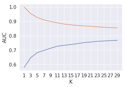
Here K=21 is the best hyperparameter as we can observe in the above graph.
#training the model with best K that we have obtained
k_tfidf=21
knn_tfidf=KNeighborsClassifier(n_neighbors=k_tfidf,algorithm='brute')
knn_tfidf.fit(train_tfidf,ytrain)
tfidf_pred=knn_tfidf.predict_proba(test_tfidf)
#deriving discrete class for plotting confusion matrix
tfidf_pred_cm = np.argmax(tfidf_pred, axis=1)
tfidf_pred=tfidf_pred[:,1]
tfidf_pred_train=knn_tfidf.predict_proba(train_tfidf)
tfidf_pred_cm_train = np.argmax(tfidf_pred_train, axis=1)
tfidf_pred_train=tfidf_pred_train[:,1]
auc_tfidf=roc_auc_score(ytest,tfidf_pred)
fpr_train, tpr_train, thresholds = roc_curve(ytrain, tfidf_pred_train)
fpr_test, tpr_test, thresholds = roc_curve(ytest, tfidf_pred)
KNN brute on Average Word2Vec
algo='brute'
krange=30
njobs=-1 #use all available cpu core
k_plot_avgw2v,auc_cv_plot_avgw2v,auc_train_plot_avgw2v=find_best_k(train_avgw2v,crossvalidation_avgw2v,algo,krange,njobs)
plt.plot(k_plot_avgw2v,auc_cv_plot_avgw2v)
plt.plot(k_plot_avgw2v,auc_train_plot_avgw2v)
plt.xlabel("K")
plt.ylabel("AUC")
plt.xticks(np.arange(min(k_plot_avgw2v), max(k_plot_avgw2v)+1, 2.0))
plt.show()

#training the model with best K that we have obtained
k_avgw2v=21
knn_avgw2v=KNeighborsClassifier(n_neighbors=k_avgw2v,algorithm='brute',n_jobs=-1)
knn_avgw2v.fit(train_avgw2v,ytrain)
avgw2v_pred=knn_avgw2v.predict_proba(test_avgw2v)
#deriving discrete class for plotting confusion matrix
avgw2v_pred_cm = np.argmax(avgw2v_pred, axis=1)
avgw2v_pred=avgw2v_pred[:,1]
#training predictions
avgw2v_pred_train=knn_avgw2v.predict_proba(train_avgw2v)
avgw2v_pred_cm_train = np.argmax(avgw2v_pred_train, axis=1)
avgw2v_pred_train=avgw2v_pred_train[:,1]
#calculating AUC on test data
auc_avgw2v=roc_auc_score(ytest,avgw2v_pred)
#roc for train data
fpr_train, tpr_train, thresholds = roc_curve(ytrain, avgw2v_pred_train)
#roc for test data
fpr_test, tpr_test, thresholds = roc_curve(ytest, avgw2v_pred)
KNN brute TF-IDF Word2Vec
algo='brute'
krange=30
njobs=-1 #use all available CPU core
k_plot_tfidfw2v,auc_cv_plot_tfidfw2v,auc_train_plot_tfidfw2v=find_best_k(train_tfidfw2v,crossvalidation_tfidfw2v,algo,krange,njobs)
plt.plot(k_plot_tfidfw2v,auc_cv_plot_tfidfw2v)
plt.plot(k_plot_tfidfw2v,auc_train_plot_tfidfw2v)
plt.xlabel("K")
plt.ylabel("AUC")
plt.xticks(np.arange(min(k_plot_tfidfw2v), max(k_plot_tfidfw2v)+1, 2.0))
plt.show()
k_tfidfw2v=23
knn_tfidfw2v=KNeighborsClassifier(n_neighbors=k_tfidfw2v,algorithm='brute',n_jobs=-1)
knn_tfidfw2v.fit(train_tfidfw2v,ytrain)
tfidfw2v_pred=knn_tfidfw2v.predict_proba(test_tfidfw2v)
#deriving discrete class for plotting confusion matrix
tfidfw2v_pred_cm = np.argmax(tfidfw2v_pred, axis=1)
tfidfw2v_pred=tfidfw2v_pred[:,1]
#training predictions
tfidfw2v_pred_train=knn_tfidfw2v.predict_proba(train_tfidfw2v)
tfidfw2v_pred_cm_train = np.argmax(tfidfw2v_pred_train, axis=1)
tfidfw2v_pred_train=tfidfw2v_pred_train[:,1]
auc_tfidfw2v=roc_auc_score(ytest,tfidfw2v_pred)
fpr_train, tpr_train, thresholds = roc_curve(ytrain, tfidfw2v_pred_train)
fpr_test, tpr_test, thresholds =roc_curve(ytest, tfidfw2v_pred)
KNN kd-tree on BOW
Here in the kd-tree approach, we will use a method called ‘TruncatedSVD’ to reduce the dimensionality of the dataset. We are doing this because the tree method can take a huge time to train on high-dimensional data.
from sklearn.decomposition import TruncatedSVD
no_of_components=500
tsvd=TruncatedSVD(n_components=no_of_components)
tsvd_train_bow=tsvd.fit_transform(train_bow)
tsvd_test_bow=tsvd.transform(test_bow)
tsvd_crossvalidation_bow=tsvd.transform(crossvalidation_bow)
algo='kd_tree'
krange=30
njobs=-1 #use all available cpu cores
kdtree_k_plot_bow,kdtree_auc_cv_plot_bow,kdtree_auc_train_plot_bow=find_best_k(tsvd_train_bow,tsvd_crossvalidation_bow,algo,krange,njobs)
plt.plot(kdtree_k_plot_bow,kdtree_auc_cv_plot_bow)
plt.plot(kdtree_k_plot_bow,kdtree_auc_train_plot_bow)
plt.xlabel("K")
plt.ylabel("AUC")
plt.xticks(np.arange(min(kdtree_k_plot_bow), max(kdtree_k_plot_bow)+1, 2.0))
plt.show()
Similarly, we built all other approaches, and below are the result that we observed.
Conclusion
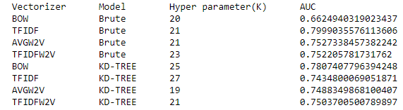
We find out that TFIDF with Bruteforce gives a maximum of AUC 0.799 with hyperparameter K=21 than any other model.
Read more articles on our blog.
The media shown in this article is not owned by Analytics Vidhya and are used at the Author’s discretion.


