Moments in Statistics – A Must Known Statistical Concept for Data Science
Statistical Moments play a crucial role when we specify our probability distribution to work with since, with the help of moments, we can describe the properties of statistical distribution. Therefore, they help define the distribution. We required the statistical moments in Statistical Estimation and Testing of Hypotheses, which all are based on the numerical values arrived for each distribution. In this article, we will discuss moments in Statistics in detail.
This article was published as a part of the Data Science Blogathon.
Table of contents
What is Moment in Statistics?
In Statistics, Moments are popularly used to describe the characteristic of a distribution. Let’s say the random variable of our interest is X then, moments are defined as the X’s expected values.
For Example, E(X), E(X²), E(X³), E(X⁴),…, etc.
Use of Moment in Statistics
- These are very useful in statistics because they tell you much about your data.
- The four commonly used moments in statistics are- the mean, variance, skewness, and kurtosis.
To be ready to compare different data sets we will describe them using the primary four statistical moments.
The First Moment
- The first central moment is the expected value, known also as an expectation, mathematical expectation, mean, or average.
- It measures the location of the central point.
Case-1: When all outcomes have the same probability of occurrence
It is defined as the sum of all the values the variable can take times the probability of that
value occurring. Intuitively, we can understand this as the arithmetic mean.
Case-2: When all outcomes don’t have the same probability of occurrence
This is the more general equation that includes the probability of each outcome and is defined as the summation of all the variables multiplied by the corresponding probability.
Conclusion
For equally probable events, the expected value is exactly the same as the Arithmetic Mean. This is one of the most popular measures of central tendency, which we also called Averages. But, there are some other common measures also like, Median and Mode.
- Median — The middle value
- Mode — The most likely value.
The Second Moment
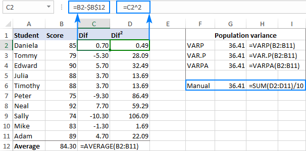
- The second central moment is “Variance”.
- It measures the spread of values in the distribution OR how far from the normal.
- Variance represents how a set of data points are spread out around their mean value.
For Example, for a sample dataset, you can find the variance as mentioned below:
Standard Deviation
Standard deviation is just a square root of the variance and is commonly used since the unit
of random variable X and Standard deviation is the same, so interpretation is easier.
For Example, For a normal distribution:
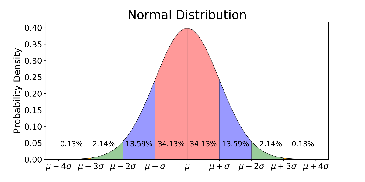
- 1 st Standard Deviation: 68.27% of the data points lie
- 2 nd Standard Deviation: 95.45% of the data points lie
- 3 rd Standard Deviation: 99.73% of the data points lie
Now. let’s understand the answer to the given questions:
Why Variance is preferred over Mean Absolute Deviation(MAD)?
Variance is preferred over MAD due to the following reasons:
Mathematical properties: The function of variance in both Continuous and differentiable.
For a Population, the Standard Deviation of a sample is a more consistent estimate: If we picked the repeated samples from a normally distributed population, then the standard deviations of samples are less spread out as compared to mean
absolute deviations.
The Third Moment
- The third statistical moment is “Skewness”.
- It measures how asymmetric the distribution is about its mean.
We can differentiate three types of distribution with respect to its skewness:
Symmetrical Distribution
If both tails of a distribution are symmetrical, and the skewness is equal to zero, then that distribution is symmetrical.
Positively Skewed
In these types of distributions, the right tail (with larger values) is longer. So, this also tells us about ‘outliers’ that have values higher than the mean. Sometimes, this is also referred to as:
- Right-skewed
- Right-tailed
- Skewed to the Right
Negatively Skewed
In these types of distributions, the left tail (with small values) is longer. So, this also tells us about ‘outliers’ that have values lower than the mean. Sometimes, this is also referred to as:
- Left-skewed
- Left-tailed
- Skewed to the Left
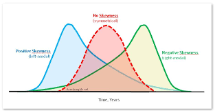
For Example, For a Normal Distribution, which is Symmetric, the value of Skewness equals 0 and that distribution is symmetrical.
In general, Skewness will impact the relationship of mean, median, and mode in the described manner:
- For a Symmetrical distribution: Mean = Median = Mode
- For a positively skewed distribution: Mode < Median < Mean (large tail of high values)
- For a negatively skewed distribution: Mean < Median < Mode (large tail of small values)
But the above generalization is not true for all possible distributions.
For Example, if one tail is long, but the other is heavy, this may not work. The best way to explore your data is to first compute all three estimators and then try to draw conclusions based on the results, rather than just focusing on the general rules.
Other Formula of Calculating Skewness
Skewness = (Mean-Mode)/SD = 3*(Mean-Median)/SD
Since, (Mode = 3*Median-2*Mean)
Some transformations to make the distribution normal:
For Positively skewed (right): Square root, log, inverse, etc.
For Negatively skewed (left): Reflect and square[sqrt(constant-x)], reflect and log, reflect
and inverse, etc.
The Fourth Moment
- The fourth statistical moment is “kurtosis”.
- It measures the amount in the tails and outliers.
- It focuses on the tails of the distribution and explains whether the distribution is flat or rather with a high peak. This measure informs us whether our distribution is richer in extreme values than the normal distribution.
For Example, For a normal distribution, the value of Kurtosis equals 3
For Kurtosis not equal to 3, there are the following cases:
- Kurtosis<3 [Lighter tails]: Negative kurtosis indicates a broad flat distribution.
- Kurtosis>3 [Heavier tails]: Positive kurtosis indicates a thin pointed distribution.
In general, we can differentiate three types of distributions based on the Kurtosis:
Mesokurtic
These types of distributions are having the kurtosis of 3 or excess kurtosis of 0. This category includes the normal distribution and some specific binomial distributions.
Leptokurtic
These types of distributions are having a kurtosis greater than 3, or excess kurtosis greater than 0. This is the distribution with fatter tails and a more narrow peak.
Platykurtic
These types of distributions are having the kurtosis smaller than 3 or excess kurtosis less than 0(negative). This is a distribution with very thin tails compared to the normal distribution.
Now, let’s define what is Excess Kurtosis
Excess Kurtosis = Kurtosis – 3
Understanding of Kurtosis related to Outliers:
- Kurtosis is defined as the average of the standardized data raised to the fourth power. Any standardized values less than |1| (i.e. data within one standard deviation of the mean) will contribute petty to kurtosis.
- The standardized values that will contribute immensely are the outliers.
- Therefore, the high value of Kurtosis alerts about the presence of outliers.
Different Types of Moments
Let’s discuss three different types of moments:
Raw Moments
The raw moment or the n-th moment about zero of a probability density function f(x) is the expected value of X^n. It is also known as the Crude moment.
Centered Moments
A central moment is a moment of a probability distribution of a random variable defined about the mean of the random variable’s i.e, it is the expected value of a specified integer power of the deviation of the random variable from the mean.
Standardized Moments
A standardized moment of a probability distribution is a moment that is normally a higher degree central moment, but it is normalized typically by dividing the standard deviation which renders the moment scale-invariant.
Python Code Examples to Calculate Moments
Here are some examples to calculate moments in statistics:
First Moment (Mean)
import numpy as np

data = [10, 12, 15, 20, 25]

mean = np.mean(data)
print("Mean:", mean)
Output
Mean: 16.4Second Moment (Variance)
import numpy as np

data = [10, 12, 15, 20, 25]

variance = np.var(data)
print("Variance:", variance)
Output
Variance: 29.839999999999996
Third Moment (Skewness)
import numpy as np
from scipy.stats import skew

data = [10, 12, 15, 20, 25]

skewness = skew(data)
print("Skewness:", skewness)
Output
Skewness: 0.4081372552079214Fourth Moment (Kurtosis)
import numpy as np
from scipy.stats import kurtosis

data = [10, 12, 15, 20, 25]

kurt = kurtosis(data)
print("Kurtosis:", kurt)
Output
Kurtosis: -1.2717442086121507
End Note
Moments in statistics are an essential statistical concept that every data scientist should know. They provide valuable insights into data distribution and help understand its central tendency, spread, and shape. By understanding moments, data scientists can make informed data analysis and modeling decisions. Whether calculating the mean and variance or exploring higher-order moments, a solid grasp of moments is crucial for accurately interpreting and manipulating data. Incorporating moments into your data science toolkit will enhance your ability to extract meaningful information and derive valuable insights from datasets. Embrace the power of moments and elevate your data science skills to new heights. You can read the following articles to learn other essential statistics functions:
Frequently Asked Questions
A. The formula for the moment in statistics depends on the order of the moment. For example, the first moment (mean) formula is Σ(xi)/n, where xi is each value in the dataset and n is the number of data points.
A. Moments in probability theory are mathematical quantities used to describe the shape and characteristics of probability distributions. They provide insights into random variables’ behavior and help quantify properties like central tendency and dispersion.
A. Moments in statistics are called moments because they capture a distribution’s “essence” or “character.” The term “moment” comes from Latin, meaning “movement” or “force.” Moments capture the movement or tendency of data points away from a reference point (such as the mean) and provide information about the distribution’s shape and properties.
A. The 5th moment in statistics refers to the fifth-order moment, which provides information about the shape and asymmetry of a distribution. It quantifies the distribution’s departure from symmetry and can indicate the presence of heavy tails or skewness.
The media shown in this article is not owned by Analytics Vidhya and are used at the Author’s discretion.
I am currently pursuing my Bachelor of Technology (B.Tech) in Computer Science and Engineering from the Indian Institute of Technology Jodhpur(IITJ). I am very enthusiastic about Machine learning, Deep Learning, and Artificial Intelligence. Feel free to connect with me on Linkedin.


