Introduction
It happened a few years back. After working on SAS for more than 5 years, I decided to move out of my comfort zone. Being a data scientist, my hunt for other useful tools was ON! Fortunately, it didn’t take me long to decide – Python was my appetizer.
I always had an inclination for coding. This was the time to do what I really loved. Code. Turned out, coding was actually quite easy!
I learned the basics of Python within a week. And, since then, I’ve not only explored this language to the depth, but also have helped many other to learn this language. Python was originally a general purpose language. But, over the years, with strong community support, this language got dedicated library for data analysis and predictive modeling.
Due to lack of resource on python for data science, I decided to create this tutorial to help many others to learn python faster. In this tutorial, we will take bite sized information about how to use Python for Data Analysis, chew it till we are comfortable and practice it at our own end. A complete python tutorial from scratch in data science.
Learning Objectives
- This article is a complete tutorial to learn data science using python from scratch
- It will also help you to learn basic data analysis methods using python
- You will also be able to enhance your knowledge of machine learning algorithms
Table of contents
You can also check out the ‘Introduction to Data Science‘ course – a comprehensive introduction to the world of data science. It includes modules on Python, Statistics and Predictive Modeling along with multiple practical projects to get your hands dirty.
Basics of Python for Data Analysis
Why learn Python for data analysis?
Python has gathered a lot of interest recently as a choice of language for data analysis. I had basics of Python some time back. Here are some reasons which go in favour of learning Python:
- Open Source – free to install
- Awesome online community
- Very easy to learn
- Can become a common language for data science and production of web based analytics products.
Needless to say, it still has few drawbacks too:
- It is an interpreted language rather than compiled language – hence might take up more CPU time. However, given the savings in programmer time (due to ease of learning), it might still be a good choice.
Python 2.7 v/s 3.4
This is one of the most debated topics in Python. You will invariably cross paths with it, specially if you are a beginner. There is no right/wrong choice here. It totally depends on the situation and your need to use. I will try to give you some pointers to help you make an informed choice.
Why Python 2.7?
- Awesome community support! This is something you’d need in your early days. Python 2 was released in late 2000 and has been in use for more than 15 years.
- Plethora of third-party libraries! Though many libraries have provided 3.x support but still a large number of modules work only on 2.x versions. If you plan to use Python for specific applications like web-development with high reliance on external modules, you might be better off with 2.7.
- Some of the features of 3.x versions have backward compatibility and can work with 2.7 version.
Why Python 3.4?
- Cleaner and faster! Python developers have fixed some inherent glitches and minor drawbacks in order to set a stronger foundation for the future. These might not be very relevant initially, but will matter eventually.
- It is the future! 2.7 is the last release for the 2.x family and eventually everyone has to shift to 3.x versions. Python 3 has released stable versions for past 5 years and will continue the same.
There is no clear winner but I suppose the bottom line is that you should focus on learning Python as a language. Shifting between versions should just be a matter of time. Stay tuned for a dedicated article on Python 2.x vs 3.x in the near future!
Are you a beginner looking for a place to start your journey in data science and machine learning? Presenting a comprehensive course, full of knowledge and data science learning, curated just for you! Certified AI & ML Blackbelt+ Program.
How to install Python?
There are 2 approaches to install Python:
- Download Python
You can download Python directly from its project site and install individual components and libraries you want
- Install Package
Alternately, you can download and install a package, which comes with pre-installed libraries. I would recommend downloading Anaconda. Another option could be Enthought Canopy Express.
Second method provides a hassle free installation and hence I’ll recommend that to beginners
The imitation of this approach is you have to wait for the entire package to be upgraded, even if you are interested in the latest version of a single library. It should not matter until and unless, until and unless, you are doing cutting edge statistical research.
Choosing a development environment
Once you have installed Python, there are various options for choosing an environment. Here are the 3 most common options:
- Terminal / Shell based
- IDLE (default environment)
- iPython notebook – similar to markdown in R
IDLE editor for Python

While the right environment depends on your need, I personally prefer iPython Notebooks a lot. It provides a lot of good features for documenting while writing the code itself and you can choose to run the code in blocks (rather than the line by line execution)
We will use iPython environment for this complete tutorial.
Warming up: Running your first Python program
You can use Python as a simple calculator to start with:
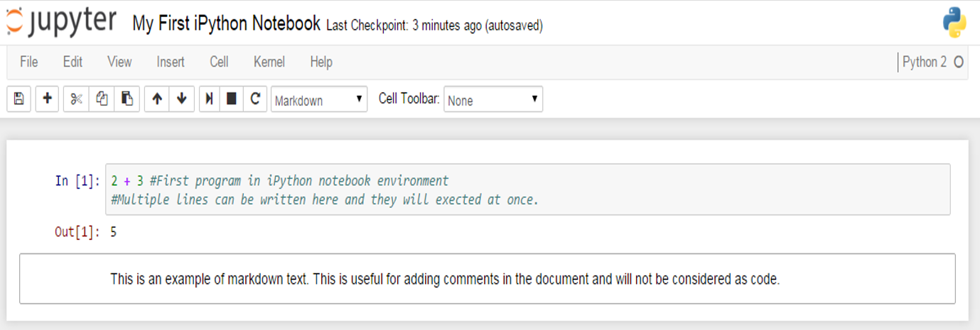
Few things to note
- You can start iPython notebook by writing “ipython notebook” on your terminal / cmd, depending on the OS you are working on
- You can name a iPython notebook by simply clicking on the name – UntitledO in the above screenshot
- The interface shows In [*] for inputs and Out[*] for output.
- You can execute a code by pressing “Shift + Enter” or “ALT + Enter”, if you want to insert an additional row after.
Before we deep dive into problem solving, lets take a step back and understand the basics of Python. As we know that data structures and iteration and conditional constructs form the crux of any language. In Python, these include lists, strings, tuples, dictionaries, for-loop, while-loop, if-else, etc. Let’s take a look at some of these.
Python libraries and Data Structures
Python Data Structures
Following are some data structures, which are used in Python. You should be familiar with them in order to use them as appropriate.
- Lists – Lists are one of the most versatile data structure in Python. A list can simply be defined by writing a list of comma separated values in square brackets. Lists might contain items of different types, but usually the items all have the same type. Python lists are mutable and individual elements of a list can be changed.
Here is a quick example to define a list and then access it:
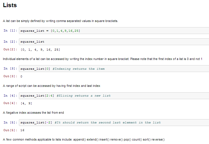
'''
PYTHON FOR DATA SCIENCE - LISTS
'''

square_list = [0, 1, 4, 9, 16, 25]
print('\n\nList = ',square_list)

'''Individual items can be accessed by index'''
#Indexing returns the items
print('\n\nItem at Index 0 = ',square_list[0])


'''slicing of list'''
# a range of items can be accessed by providing the first and last index
print('\n\n Items from index 2 to 4 = ', square_list[2:4])


'''Access elements from end with negative index'''
print('\n\nThe second last element of the list is :', square_list[-2])- Strings – Strings can simply be defined by use of single ( ‘ ), double ( ” ) or triple ( ”’ ) inverted commas. Strings enclosed in tripe quotes ( ”’ ) can span over multiple lines and are used frequently in docstrings (Python’s way of documenting functions). \ is used as an escape character. Please note that Python strings are immutable, so you can not change part of strings.
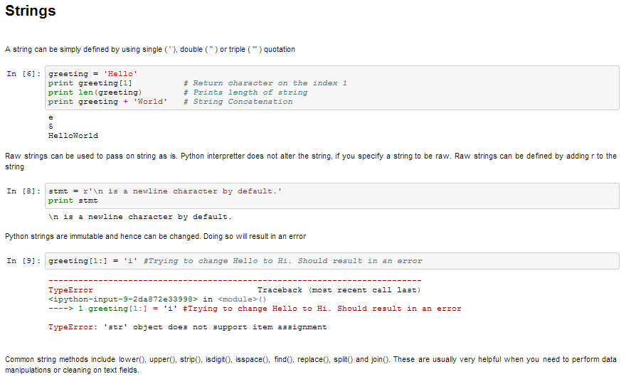
'''
PYTHON FOR DATA SCIENCE - STRINGS
'''

# define a string Value
my_string = 'Hello'

# character at index 1
print('Character at index 1 = ', my_string[1])

# length of the string
print('\n\nLength of the string = ', len(my_string))

# string concatenation
new_string = my_string+' World'
print('\n\nnew String is = ',new_string)- Tuples – A tuple is represented by a number of values separated by commas. Tuples are immutable and the output is surrounded by parentheses so that nested tuples are processed correctly. Additionally, even though tuples are immutable, they can hold mutable data if needed.
Since Tuples are immutable and can not change, they are faster in processing as compared to lists. Hence, if your list is unlikely to change, you should use tuples, instead of lists.
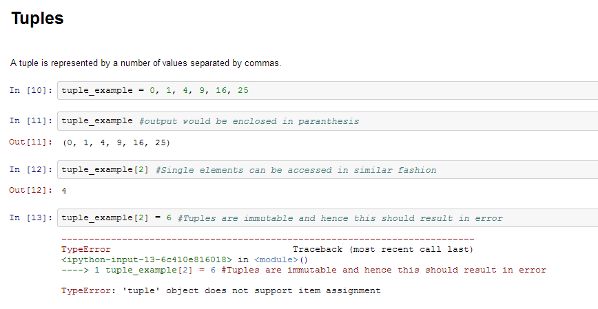
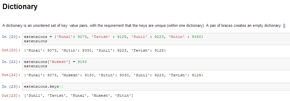
- Dictionary – Dictionary is an unordered set of key: value pairs, with the requirement that the keys are unique (within one dictionary). A pair of braces creates an empty dictionary: {}.
'''
PYTHON FOR DATA SCIENCE - TUPLES AND DICTIONARY
'''

# define a tuple
my_tuple = (1, 2, 3, 4, 5)

# access single element using index
print('TUPLE = ',my_tuple)

print('\n\nelement at index 1 = ',my_tuple[1])

# uncomment the below code and you see the error as the tuples are immutable
#my_tuple[2] = 4

# define a dictionary
my_dict = {
  'key_1' : 4,
  'key_2' : 5,
  'key_3' : 6,
  'key_4' : 7
}

# access value of any key
print('\n\nThe value of key_1 in the dictionary is ',my_dict['key_1'])

# dictionaries are mutable
my_dict['key_1'] = 1000

print('\n\nThe value of key_1 after update in the dictionary is ',my_dict['key_1'])


#keys of dictionary
print('\n\nkeys = ',my_dict.keys())
Python Iteration and Conditional Constructs
Like most languages, Python also has a FOR-loop which is the most widely used method for iteration. It has a simple syntax:
for i in [Python Iterable]:
  expression(i)
Here “Python Iterable” can be a list, tuple or other advanced data structures which we will explore in later sections. Let’s take a look at a simple example, determining the factorial of a number.
fact=1
for i in range(1,N+1):
  fact *= i
Coming to conditional statements, these are used to execute code fragments based on a condition. The most commonly used construct is if-else, with following syntax:
if [condition]:
  __execution if true__
else:
  __execution if false__
For instance, if we want to print whether the number N is even or odd:
if N%2 == 0:
  print ('Even')
else:
  print ('Odd')
Now that you are familiar with Python fundamentals, let’s take a step further. What if you have to perform the following tasks:
- Multiply 2 matrices
- Find the root of a quadratic equation
- Plot bar charts and histograms
- Make statistical models
- Access web-pages
If you try to write code from scratch, its going to be a nightmare and you won’t stay on Python for more than 2 days! But lets not worry about that. Thankfully, there are many libraries with predefined which we can directly import into our code and make our life easy.
For example, consider the factorial example we just saw. We can do that in a single step as:
math.factorial(N)Off-course we need to import the math library for that. Lets explore the various libraries next.
Python Libraries
Lets take one step ahead in our journey to learn Python by getting acquainted with some useful libraries. The first step is obviously to learn to import them into our environment. There are several ways of doing so in Python:
import math as mfrom math import *In the first manner, we have defined an alias m to library math. We can now use various functions from math library (e.g. factorial) by referencing it using the alias m.factorial().
In the second manner, you have imported the entire name space in math i.e. you can directly use factorial() without referring to math.
Tip: Google recommends that you use first style of importing libraries, as you will know where the functions have come from.
List of Top Python Libraries for Data Science
Following are a list of libraries, you will need for any scientific computations and data analysis:
| Library | Description |
|---|---|
| NumPy | Powerful for n-dimensional arrays, linear algebra, Fourier transforms, and integration with other languages. |
| SciPy | Built on NumPy, ideal for science and engineering tasks like Fourier transforms, Linear Algebra, and Optimization. |
| Matplotlib | Versatile plotting, from histograms to heat plots. Offers inline plotting and supports LaTeX commands for math. |
| Pandas | Essential for structured data operations, widely used in data munging and preparation for data science. |
| Scikit Learn | Efficient tools for machine learning and statistical modeling, including classification, regression, and clustering. |
| Statsmodels | For statistical modeling, provides descriptive statistics, tests, and plotting functions across various data types. |
| Seaborn | Aims for attractive statistical data visualization, built on Matplotlib, making exploration and understanding of data central. |
| Bokeh | Creates interactive plots, dashboards, and data applications for modern web browsers, with high-performance interactivity. |
| Blaze | Extends NumPy and Pandas capabilities to distributed and streaming datasets, accessing data from various sources. |
| Scrapy | Web crawling framework, useful for extracting specific data patterns by navigating through web-pages within a website. |
| SymPy | For symbolic computation, covers arithmetic to quantum physics, with the capability to format results as LaTeX code. |
| Requests | Simplifies web access compared to urllib2, convenient for beginners with slight differences. |
Additional Libraries
- os for Operating system and file operations
- networkx and igraph for graph based data manipulations
- regular expressions for finding patterns in text data
- BeautifulSoup for scrapping web. It is inferior to Scrapy as it will extract information from just a single webpage in a run.
Now that we are familiar with Python fundamentals and additional libraries, lets take a deep dive into problem solving through Python. Yes I mean making a predictive model! In the process, we use some powerful libraries and also come across the next level of data structures. We will take you through the 3 key phases:
- Data Exploration – finding out more about the data we have
- Data Munging – cleaning the data and playing with it to make it better suit statistical modeling
- Predictive Modeling – running the actual algorithms and having fun 🙂
Exploratory analysis in Python using Pandas
In order to explore our data further, let me introduce you to another animal (as if Python was not enough!) – Pandas.
Pandas is one of the most useful data analysis library in Python (I know these names sounds weird, but hang on!). They have been instrumental in increasing the use of Python in data science community. We will now use Pandas to read a data set from an Analytics Vidhya competition, perform exploratory analysis and build our first basic categorization algorithm for solving this problem.
Before loading the data, lets understand the 2 key data structures in Pandas – Series and DataFrames
Introduction to Series and Dataframes
Series can be understood as a 1 dimensional labelled / indexed array. You can access individual elements of this series through these labels.
A dataframe is similar to Excel workbook – you have column names referring to columns and you have rows, which can be accessed with use of row numbers. The essential difference being that column names and row numbers are known as column and row index, in case of dataframes.
Series and dataframes form the core data model for Pandas in Python. The data sets are first to read into these dataframes and then various operations (e.g. group by, aggregation etc.) can be applied very easily to its columns.
More: 10 Minutes to Pandas
Practice data set – Loan Prediction Problem
You can download the dataset from here. Here is the description of the variables:
VARIABLE DESCRIPTIONS:
Variable	          Description
Loan_ID	                  Unique Loan ID
Gender	                  Male/ Female
Married	                  Applicant married (Y/N)
Dependents	          Number of dependents
Education	          Applicant Education (Graduate/ Under Graduate)
Self_Employed	          Self employed (Y/N)
ApplicantIncome	          Applicant income
CoapplicantIncome	  Coapplicant income
LoanAmount	          Loan amount in thousands
Loan_Amount_Term	  Term of loan in months
Credit_History	          credit history meets guidelines
Property_Area	          Urban/ Semi Urban/ Rural
Loan_Status	          Loan approved (Y/N)
Let’s begin with the exploration
To begin, start iPython interface in Inline Pylab mode by typing following on your terminal/windows command prompt:
ipython notebook --pylab=inlineThis opens up iPython notebook in pylab environment, which has a few useful libraries already imported. Also, you will be able to plot your data inline, which makes this a really good environment for interactive data analysis. You can check whether the environment has loaded correctly, by typing the following command (and getting the output as seen in the figure below):
plot(arange(5))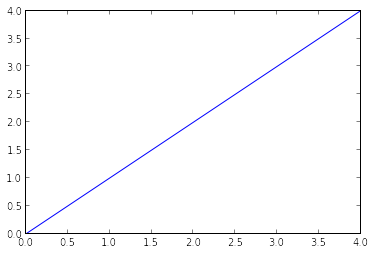
I am currently working in Linux, and have stored the dataset in the following location:
/home/kunal/Downloads/Loan_Prediction/train.csv
Importing libraries and the data set:
Following are the libraries we will use during this tutorial:
- numpy
- matplotlib
- pandas
Please note that you do not need to import matplotlib and numpy because of Pylab environment. I have still kept them in the code, in case you use the code in a different environment.
After importing the library, you read the dataset using function read_csv(). This is how the code looks like till this stage:
import pandas as pd
import numpy as np
import matplotlib as plt
%matplotlib inline

df = pd.read_csv("/home/kunal/Downloads/Loan_Prediction/train.csv") #Reading the dataset in a dataframe using Pandas
Quick Data Exploration
Once you have read the dataset, you can have a look at few top rows by using the function head()
df.head(10)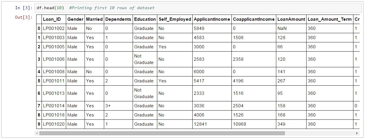
This should print 10 rows. Alternately, you can also look at more rows by printing the dataset.
Next, you can look at summary of numerical fields by using describe() function
df.describe()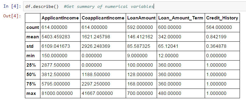
describe() function would provide count, mean, standard deviation (std), min, quartiles and max in its output (Read this article to refresh basic statistics to understand population distribution)
Here are a few inferences, you can draw by looking at the output of describe() function:
- LoanAmount has (614 – 592) 22 missing values.
- Loan_Amount_Term has (614 – 600) 14 missing values.
- Credit_History has (614 – 564) 50 missing values.
- We can also look that about 84% applicants have a credit_history. How? The mean of Credit_History field is 0.84 (Remember, Credit_History has value 1 for those who have a credit history and 0 otherwise)
- The ApplicantIncome distribution seems to be in line with expectation. Same with CoapplicantIncome
Please note that we can get an idea of a possible skew in the data by comparing the mean to the median, i.e. the 50% figure.
For the non-numerical values (e.g. Property_Area, Credit_History etc.), we can look at frequency distribution to understand whether they make sense or not. The frequency table can be printed by following command:
df['Property_Area'].value_counts()Similarly, we can look at unique values of port of credit history. Note that dfname[‘column_name’] is a basic indexing technique to acess a particular column of the dataframe. It can be a list of columns as well. For more information, refer to the “10 Minutes to Pandas” resource shared above.
Distribution analysis
Now that we are familiar with basic data characteristics, let us study distribution of various variables. Let us start with numeric variables – namely ApplicantIncome and LoanAmount
Lets start by plotting the histogram of ApplicantIncome using the following commands:
df['ApplicantIncome'].hist(bins=50)
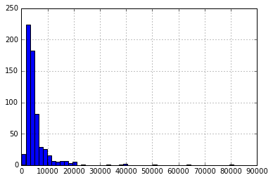
Here we observe that there are few extreme values. This is also the reason why 50 bins are required to depict the distribution clearly.
Next, we look at box plots to understand the distributions. Box plot for fare can be plotted by:
df.boxplot(column='ApplicantIncome')
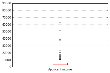
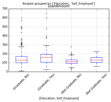
This confirms the presence of a lot of outliers/extreme values. This can be attributed to the income disparity in the society. Part of this can be driven by the fact that we are looking at people with different education levels. Let us segregate them by Education:
df.boxplot(column='ApplicantIncome', by = 'Education')
We can see that there is no substantial different between the mean income of graduate and non-graduates. But there are a higher number of graduates with very high incomes, which are appearing to be the outliers.
Now, Let’s look at the histogram and boxplot of LoanAmount using the following command:
df['LoanAmount'].hist(bins=50)

 df.boxplot(column='LoanAmount')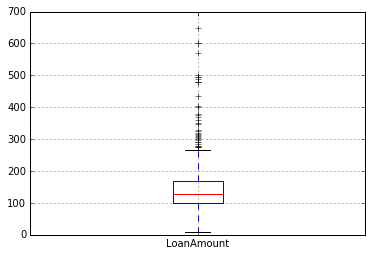
Again, there are some extreme values. Clearly, both ApplicantIncome and LoanAmount require some amount of data munging. LoanAmount has missing and well as extreme values values, while ApplicantIncome has a few extreme values, which demand deeper understanding. We will take this up in coming sections.
Categorical variable analysis
Now that we understand distributions for ApplicantIncome and LoanIncome, let us understand categorical variables in more details. We will use Excel style pivot table and cross-tabulation. For instance, let us look at the chances of getting a loan based on credit history. This can be achieved in MS Excel using a pivot table as:
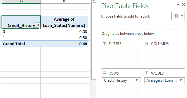
Note: here loan status has been coded as 1 for Yes and 0 for No. So the mean represents the probability of getting loan.
Now we will look at the steps required to generate a similar insight using Python. Please refer to this article for getting a hang of the different data manipulation techniques in Pandas.
temp1 = df['Credit_History'].value_counts(ascending=True)
temp2 = df.pivot_table(values='Loan_Status',index=['Credit_History'],aggfunc=lambda x: x.map({'Y':1,'N':0}).mean())
print ('Frequency Table for Credit History:')
print (temp1)

print ('\nProbility of getting loan for each Credit History class:')
print (temp2)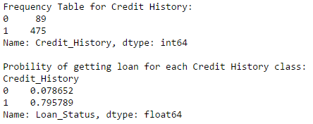
Now we can observe that we get a similar pivot_table like the MS Excel one. This can be plotted as a bar chart using the “matplotlib” library with following code:
import matplotlib.pyplot as plt
fig = plt.figure(figsize=(8,4))
ax1 = fig.add_subplot(121)
ax1.set_xlabel('Credit_History')
ax1.set_ylabel('Count of Applicants')
ax1.set_title("Applicants by Credit_History")
temp1.plot(kind='bar')

ax2 = fig.add_subplot(122)
temp2.plot(kind = 'bar')
ax2.set_xlabel('Credit_History')
ax2.set_ylabel('Probability of getting loan')
ax2.set_title("Probability of getting loan by credit history")
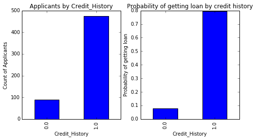
This shows that the chances of getting a loan are eight-fold if the applicant has a valid credit history. You can plot similar graphs by Married, Self-Employed, Property_Area, etc.
Alternately, these two plots can also be visualized by combining them in a stacked chart::
temp3 = pd.crosstab(df['Credit_History'], df['Loan_Status'])
temp3.plot(kind='bar', stacked=True, color=['red','blue'], grid=False)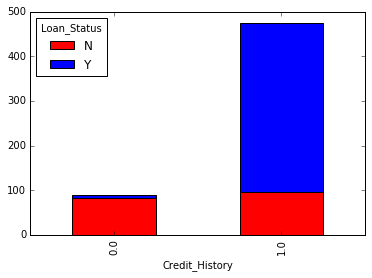
You can also add gender into the mix (similar to the pivot table in Excel):
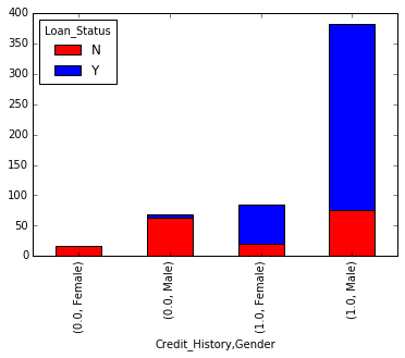
If you have not realized already, we have just created two basic classification algorithms here, one based on credit history, while other on 2 categorical variables (including gender). You can quickly code this to create your first submission on AV Datahacks.
We just saw how we can do exploratory analysis in Python using Pandas. I hope your love for pandas (the animal) would have increased by now – given the amount of help, the library can provide you in analyzing datasets.
Next let’s explore ApplicantIncome and LoanStatus variables further, perform data munging and create a dataset for applying various modeling techniques. I would strongly urge that you take another dataset and problem and go through an independent example before reading further.
Data Munging in Python : Using Pandas
For those, who have been following, here are your must wear shoes to start running.
Data munging – recap of the need
While our exploration of the data, we found a few problems in the data set, which needs to be solved before the data is ready for a good model. This exercise is typically referred as “Data Munging”. Here are the problems, we are already aware of:
- There are missing values in some variables. We should estimate those values wisely depending on the amount of missing values and the expected importance of variables.
- While looking at the distributions, we saw that ApplicantIncome and LoanAmount seemed to contain extreme values at either end. Though they might make intuitive sense, but should be treated appropriately.
In addition to these problems with numerical fields, we should also look at the non-numerical fields i.e. Gender, Property_Area, Married, Education and Dependents to see, if they contain any useful information.
If you are new to Pandas, I would recommend reading this article before moving on. It details some useful techniques of data manipulation.
Check missing values in the dataset
Let us look at missing values in all the variables because most of the models don’t work with missing data and even if they do, imputing them helps more often than not. So, let us check the number of nulls / NaNs in the dataset
df.apply(lambda x: sum(x.isnull()),axis=0)
This command should tell us the number of missing values in each column as isnull() returns 1, if the value is null.
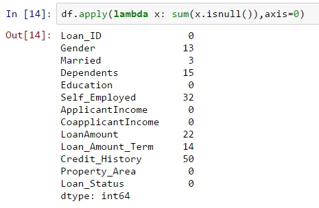
Though the missing values are not very high in number, but many variables have them and each one of these should be estimated and added in the data. Get a detailed view on different imputation techniques through this article.
Note: Remember that missing values may not always be NaNs. For instance, if the Loan_Amount_Term is 0, does it makes sense or would you consider that missing? I suppose your answer is missing and you’re right. So we should check for values which are unpractical.
How to fill missing values in LoanAmount?
There are numerous ways to fill the missing values of loan amount – the simplest being replacement by mean, which can be done by following code:
df['LoanAmount'].fillna(df['LoanAmount'].mean(), inplace=True)
The other extreme could be to build a supervised learning model to predict loan amount on the basis of other variables and then use age along with other variables to predict survival.
Since, the purpose now is to bring out the steps in data munging, I’ll rather take an approach, which lies some where in between these 2 extremes. A key hypothesis is that the whether a person is educated or self-employed can combine to give a good estimate of loan amount.
First, let’s look at the boxplot to see if a trend exists:
Thus we see some variations in the median of loan amount for each group and this can be used to impute the values. But first, we have to ensure that each of Self_Employed and Education variables should not have a missing values.
As we say earlier, Self_Employed has some missing values. Let’s look at the frequency table:
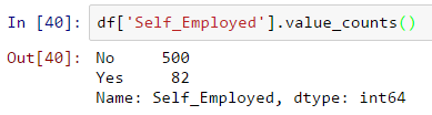
Since ~86% values are “No”, it is safe to impute the missing values as “No” as there is a high probability of success. This can be done using the following code:
df['Self_Employed'].fillna('No',inplace=True)Now, we will create a Pivot table, which provides us median values for all the groups of unique values of Self_Employed and Education features. Next, we define a function, which returns the values of these cells and apply it to fill the missing values of loan amount:
table = df.pivot_table(values='LoanAmount', index='Self_Employed' ,columns='Education', aggfunc=np.median)
# Define function to return value of this pivot_table
def fage(x):
 return table.loc[x['Self_Employed'],x['Education']]
# Replace missing values
df['LoanAmount'].fillna(df[df['LoanAmount'].isnull()].apply(fage, axis=1), inplace=True)
This should provide you a good way to impute missing values of loan amount.
NOTE : This method will work only if you have not filled the missing values in Loan_Amount variable using the previous approach, i.e. using mean.
How to treat for extreme values in distribution of LoanAmount and ApplicantIncome?
Let’s analyze LoanAmount first. Since the extreme values are practically possible, i.e. some people might apply for high value loans due to specific needs. So instead of treating them as outliers, let’s try a log transformation to nullify their effect:
df['LoanAmount_log'] = np.log(df['LoanAmount'])
df['LoanAmount_log'].hist(bins=20)
Looking at the histogram again:
Now the distribution looks much closer to normal and effect of extreme values has been significantly subsided.
Coming to ApplicantIncome. One intuition can be that some applicants have lower income but strong support Co-applicants. So it might be a good idea to combine both incomes as total income and take a log transformation of the same.
df['TotalIncome'] = df['ApplicantIncome'] + df['CoapplicantIncome']
df['TotalIncome_log'] = np.log(df['TotalIncome'])
df['LoanAmount_log'].hist(bins=20) 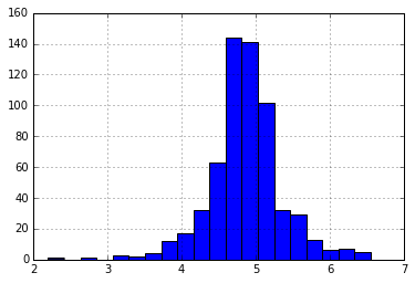
Now we see that the distribution is much better than before. I will leave it upto you to impute the missing values for Gender, Married, Dependents, Loan_Amount_Term, Credit_History. Also, I encourage you to think about possible additional information which can be derived from the data. For example, creating a column for LoanAmount/TotalIncome might make sense as it gives an idea of how well the applicant is suited to pay back his loan.
Next, we will look at making predictive models.
Building a Predictive Model in Python
After, we have made the data useful for modeling, let’s now look at the python code to create a predictive model on our data set. Skicit-Learn (sklearn) is the most commonly used library in Python for this purpose and we will follow the trail. I encourage you to get a refresher on sklearn through this article.
Since, sklearn requires all inputs to be numeric, we should convert all our categorical variables into numeric by encoding the categories. Before that we will fill all the missing values in the dataset. This can be done using the following code:
df['Gender'].fillna(df['Gender'].mode()[0], inplace=True)
df['Married'].fillna(df['Married'].mode()[0], inplace=True)
df['Dependents'].fillna(df['Dependents'].mode()[0], inplace=True)
df['Loan_Amount_Term'].fillna(df['Loan_Amount_Term'].mode()[0], inplace=True)
df['Credit_History'].fillna(df['Credit_History'].mode()[0], inplace=True)
from sklearn.preprocessing import LabelEncoder
var_mod = ['Gender','Married','Dependents','Education','Self_Employed','Property_Area','Loan_Status']
le = LabelEncoder()
for i in var_mod:
df[i] = le.fit_transform(df[i])
df.dtypes Next, we will import the required modules. Then we will define a generic classification function, which takes a model as input and determines the Accuracy and Cross-Validation scores. Since this is an introductory article, I will not go into the details of coding. Please refer to this article for getting details of the algorithms with R and Python codes. Also, it’ll be good to get a refresher on cross-validation through this article, as it is a very important measure of power performance.
 #Import models from scikit learn module:
from sklearn.linear_model import LogisticRegression
from sklearn.cross_validation import KFold   #For K-fold cross validation
from sklearn.ensemble import RandomForestClassifier
from sklearn.tree import DecisionTreeClassifier, export_graphviz
from sklearn import metrics

#Generic function for making a classification model and accessing performance:
def classification_model(model, data, predictors, outcome):
  #Fit the model:
  model.fit(data[predictors],data[outcome])

  #Make predictions on training set:
  predictions = model.predict(data[predictors])

  #Print accuracy
  accuracy = metrics.accuracy_score(predictions,data[outcome])
  print ("Accuracy : %s" % "{0:.3%}".format(accuracy))

  #Perform k-fold cross-validation with 5 folds
  kf = KFold(data.shape[0], n_folds=5)
  error = []
  for train, test in kf:
    # Filter training data
    train_predictors = (data[predictors].iloc[train,:])

    # The target we're using to train the algorithm.
    train_target = data[outcome].iloc[train]

    # Training the algorithm using the predictors and target.
    model.fit(train_predictors, train_target)

    #Record error from each cross-validation run
    error.append(model.score(data[predictors].iloc[test,:], data[outcome].iloc[test]))

  print ("Cross-Validation Score : %s" % "{0:.3%}".format(np.mean(error)))

  #Fit the model again so that it can be refered outside the function:
  model.fit(data[predictors],data[outcome])
Logistic Regression
Let’s make our first Logistic Regression model. One way would be to take all the variables into the model but this might result in overfitting (don’t worry if you’re unaware of this terminology yet). In simple words, taking all variables might result in the model understanding complex relations specific to the data and will not generalize well. Read more about Logistic Regression.
We can easily make some intuitive hypothesis to set the ball rolling. The chances of getting a loan will be higher for:
- Applicants having a credit history (remember we observed this in exploration?)
- Applicants with higher applicant and co-applicant incomes
- Applicants with higher education level
- Properties in urban areas with high growth perspectives
So let’s make our first model with ‘Credit_History’.
outcome_var = 'Loan_Status'
model = LogisticRegression()
predictor_var = ['Credit_History']
classification_model(model, df,predictor_var,outcome_var)
Accuracy : 80.945% Cross-Validation Score : 80.946%
#We can try different combination of variables:
predictor_var = ['Credit_History','Education','Married','Self_Employed','Property_Area']
classification_model(model, df,predictor_var,outcome_var)
Accuracy : 80.945% Cross-Validation Score : 80.946%
Generally we expect the accuracy to increase on adding variables. But this is a more challenging case. The accuracy and cross-validation score are not getting impacted by less important variables. Credit_History is dominating the mode. We have two options now:
- Feature Engineering: dereive new information and try to predict those. I will leave this to your creativity.
- Better modeling techniques. Let’s explore this next.
Decision Tree
Decision tree is another method for making a predictive model. It is known to provide higher accuracy than logistic regression model. Read more about Decision Trees.
model = DecisionTreeClassifier()
predictor_var = ['Credit_History','Gender','Married','Education']
classification_model(model, df,predictor_var,outcome_var)
Accuracy : 81.930% Cross-Validation Score : 76.656%
Here the model based on categorical variables is unable to have an impact because Credit History is dominating over them. Let’s try a few numerical variables:
#We can try different combination of variables:
predictor_var = ['Credit_History','Loan_Amount_Term','LoanAmount_log']
classification_model(model, df,predictor_var,outcome_var)
Accuracy : 92.345% Cross-Validation Score : 71.009%
Here we observed that although the accuracy went up on adding variables, the cross-validation error went down. This is the result of model over-fitting the data. Let’s try an even more sophisticated algorithm and see if it helps:
Random Forest
Random forest is another algorithm for solving the classification problem. Read more about Random Forest.
An advantage with Random Forest is that we can make it work with all the features and it returns a feature importance matrix which can be used to select features.
model = RandomForestClassifier(n_estimators=100)
predictor_var = ['Gender', 'Married', 'Dependents', 'Education',
       'Self_Employed', 'Loan_Amount_Term', 'Credit_History', 'Property_Area',
        'LoanAmount_log','TotalIncome_log']
classification_model(model, df,predictor_var,outcome_var)
Accuracy : 100.000% Cross-Validation Score : 78.179%
Here we see that the accuracy is 100% for the training set. This is the ultimate case of overfitting and can be resolved in two ways:
- Reducing the number of predictors
- Tuning the model parameters
Let’s try both of these. First we see the feature importance matrix from which we’ll take the most important features.
#Create a series with feature importances:
featimp = pd.Series(model.feature_importances_, index=predictor_var).sort_values(ascending=False)
print (featimp)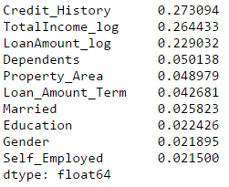
Let’s use the top 5 variables for creating a model. Also, we will modify the parameters of random forest model a little bit:
model = RandomForestClassifier(n_estimators=25, min_samples_split=25, max_depth=7, max_features=1)
predictor_var = ['TotalIncome_log','LoanAmount_log','Credit_History','Dependents','Property_Area']
classification_model(model, df,predictor_var,outcome_var)
Accuracy : 82.899% Cross-Validation Score : 81.461%
Notice that although accuracy reduced, but the cross-validation score is improving showing that the model is generalizing well. Remember that random forest models are not exactly repeatable. Different runs will result in slight variations because of randomization. But the output should stay in the ballpark.
You would have noticed that even after some basic parameter tuning on random forest, we have reached a cross-validation accuracy only slightly better than the original logistic regression model. This exercise gives us some very interesting and unique learning:
- Using a more sophisticated model does not guarantee better results.
- Avoid using complex modeling techniques as a black box without understanding the underlying concepts. Doing so would increase the tendency of overfitting thus making your models less interpretable
- Feature Engineering is the key to success. Everyone can use an Xgboost models but the real art and creativity lies in enhancing your features to better suit the model.
You can access the dataset and problem statement used in this post at this link: Loan Prediction Challenge
Projects
Now, its time to take the plunge and actually play with some other real datasets. So are you ready to take on the challenge? Accelerate your data science journey with the following Practice Problems:
 | Practice Problem: Food Demand Forecasting Challenge | Predict the demand of meals for a meal delivery company |
 | Practice Problem: HR Analytics Challenge | Identify the employees most likely to get promoted |
 | Practice Problem: Predict Number of Upvotes | Predict number of upvotes on a query asked at an online question & answer platform |
Conclusion
I hope this tutorial will help you maximize your efficiency when starting with data science in Python. I am sure this not only gave you an idea about basic data analysis methods but it also showed you how to implement some of the more sophisticated techniques available today.
You should also check out our free Python course and then jump over to learn how to apply it for Data Science.
Python is really a great tool and is becoming an increasingly popular language among the data scientists. The reason being, it’s easy to learn, integrates well with other databases and tools like Spark and Hadoop. Majorly, it has the great computational intensity and has powerful data analytics libraries.
So, learn Python to perform the full life-cycle of any data science project. It includes reading, analyzing, visualizing and finally making predictions.
If you come across any difficulty while practicing Python, or you have any thoughts /suggestions/feedback on the post, please feel free to post them through comments below.
Note – The discussions of this article are going on at AV’s Discuss portal. Join here!
If you like what you just read & want to continue your analytics learning, subscribe to our emails, follow us on twitter or like our facebook page.
Frequently Asked Questions
Q1. How to learn python programming?
A. To learn Python programming, you can start by familiarizing yourself with the language’s syntax, data types, control structures, functions, and modules. You can then practice coding by solving problems and building projects. Joining online communities, attending workshops, and taking online courses can also help you learn Python. With regular practice, persistence, and a willingness to learn, you can become proficient in Python and start developing software applications.
Q2. Why Python is used?
A. Python is used for a wide range of applications, including web development, data analysis, scientific computing, machine learning, artificial intelligence, and automation. Python is a high-level, interpreted, and dynamically-typed language that offers ease of use, readability, and flexibility. Its vast library of modules and packages makes it a popular choice for developers looking to create powerful, efficient, and scalable software applications. Python’s popularity and versatility have made it one of the most widely used programming languages in the world today.
Q3. What are the 4 basics of Python?
A. The four basics of Python are variables, data types, control structures, and functions. Variables are used to store values, data types define the type of data that can be stored, control structures dictate the flow of execution, and functions are reusable blocks of code. Understanding these four basics is essential for learning Python programming and developing software applications.
Q4. Can I teach myself Python?
A. Yes, you can teach yourself Python. Start by learning the basics and practicing coding regularly. Join online communities to get help and collaborate on projects. Building projects is a great way to apply your knowledge and develop your skills. Remember to be persistent, learn from mistakes, and keep practicing.
Kunal Jain is the Founder and CEO of Analytics Vidhya, one of the world's leading communities of Al professionals. With over 17 years of experience in the field, Kunal has been instrumental in shaping the global Al landscape. His expertise spans diverse markets, from developed economies like the UK to emerging ones like India, where he has successfully led and delivered complex data-driven solutions. As a recognized thought leader, Kunal has empowered countless individuals to realize their Al ambitions through his visionary approach to Al education and community building. Before founding Analytics Vidhya, Kunal earned both his undergraduate and postgraduate degrees from IIT Bombay and held key roles at Capital One and Aviva Life Insurance across multiple geographies. His passion lies at the intersection of analytics, Al, and fostering a thriving community of data science professionals.


can you please suggest me good data analysis book on python
There is a very good book on Python for Data Analysis, O Reily -- Python for Data Analysis
Moumita, The book mentioned by Paritosh is a good place to start. You can also refer some of the books mentioned here: http://www.analyticsvidhya.com/blog/2014/06/books-data-scientists-or-aspiring-ones/ Hope this helps. Kunal
Hi Kunal, When you are planning to schedule next data science meetup in Bangalore. I have missed the previous session due to conflict
Pranesh, We will have a meetup some time in early March. We will announce the dates on DataHack platform and our meetup group page. Hope to see you around this time. Regards, Kunal
Little error just matter for newbe as I'm: import matplotlib.pyplot as plt fig = plt.pyplot.figure(figsize=(8,4)) Error import matplotlib.pyplot as plt fig = plt.figure(figsize=(8,4)) Right
Thanks Gianfranco for highlighting it. Have corrected the same. Regards, Kunal