This article was published as a part of the Data Science Blogathon.
Over the past several years, groundbreaking developments in machine learning and artificial intelligence have reshaped the world around us. There are various deep learning algorithms that bring Machine Learning to a new level, allowing robots to learn to discriminate tasks utilizing the human brain’s neural network. Our smartphones and TV remotes have voice control because of this.
Deep learning is a machine learning approach that trains computers to learn by doing, just like people do. Using deep learning, autonomous automobiles can discriminate between a pedestrian and a lamppost, as well as a stop sign. You need this technology to use voice control on smartphones, tablets, TVs, and hands-free speakers. There’s a lot of buzz these days about deep learning, and it’s well-deserved. Achieving achievements hitherto unseen is what it’s all about.
Using deep learning, classification tasks may be learned directly from pictures, text, or voice. In some cases, deep learning algorithms can outperform humans’ inaccuracy. Large datasets of labeled data and multi-layered neural network designs are used to train models.
In a nutshell, precision. The degree of recognition accuracy achieved by deep learning has never been higher. For safety-critical applications, such as autonomous automobiles, this helps satisfy user expectations. Deep learning has recently outperformed humans when it comes to some tasks, such as identifying objects in photographs.
Several types of deep learning models are both accurate and successful at solving issues that are too complicated for the human brain to solve. This is how:
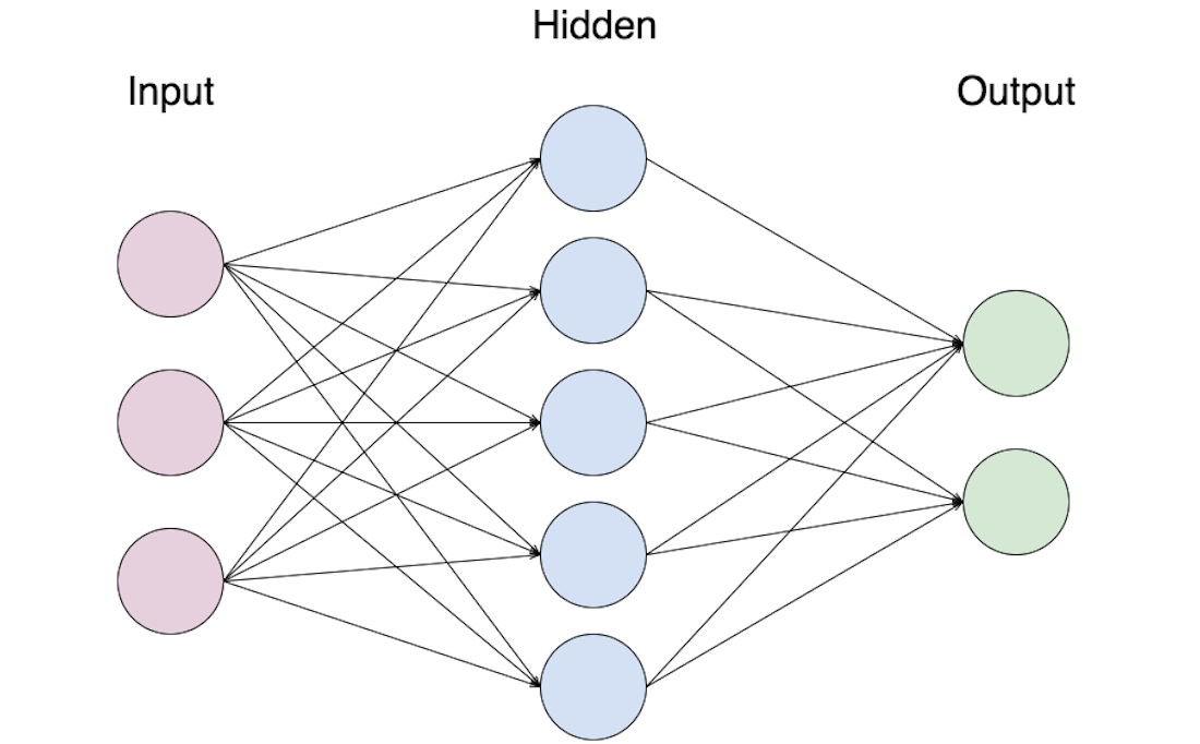
It is also known as Fully Connected Neural Networks and is distinguished by its multilayer perceptrons connected to the continuous layer. Fran Rosenblatt, an American psychologist, created it in 1958.
As a result, the model is reduced to a series of simple binary data inputs. The three functions of this model are as follows:
Linear function: As the name implies, a single line multiplies its inputs with a constant multiplier.
Non-Linear function: It is further subdivided into three subsets:
Effective in the following situations:
Any tabular dataset with CSV-formatted rows and columns
Classification and regression problems with real-valued input
Any model with a great degree of flexibility, such as ANNS
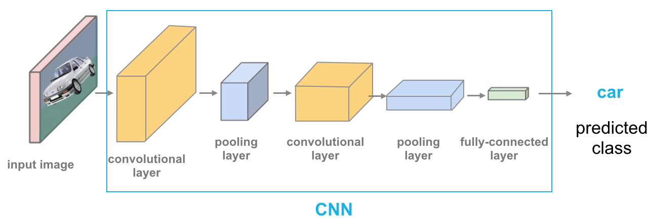
CNN is a more sophisticated and high-potential variant of the traditional artificial neural network concept. It is designed for complicated problems, preprocessing, and data compilation. It is based on the arrangement of neurons in an animal’s visual cortex.
CNNs are one of the most efficient and versatile models specializing in image and non-image data. These are divided into four distinct organizations:
Typically, it has a two-dimensional layout of neurons to understand main visual data similar to that of photo pixels.
The single-dimensional output layer of neurons in certain CNNs also analyses images on their inputs via distributed linked convolutional layers.
It’s also worth noting that CNNs contain an additional tier known as a sample layer, limiting the number of neurons in the network.
Connecting the input layer to each output layer is common in CNNs, which typically include one or more connected layers.
This network architecture may aid in extracting pertinent visual data in the form of smaller units or chunks. The neurons in the convolution layers are responsible for the preceding layer’s cluster of neurons.
After the input data is loaded into the convolutional model, the CNN is constructed in four stages:
Convolution: The technique generates feature maps from the input data and then applies a function to them.
Max-Pooling: It enables CNN to recognize images that have been modified.
Flattening: At this stage, the produced data is flattened for analysis by a CNN.
Full Connection is frequently described as a hidden layer that compiles a model’s loss function.
CNNs can perform image recognition, image analysis, image segmentation, video analysis, and natural language processing tasks. However, there may be additional instances in which CNN networks become valuable, such as the following:
OCR document analysis on image datasets
Any two-dimensional input data that can be converted to one-dimensional for faster analysis
To provide results, the model must be involved in its architecture.
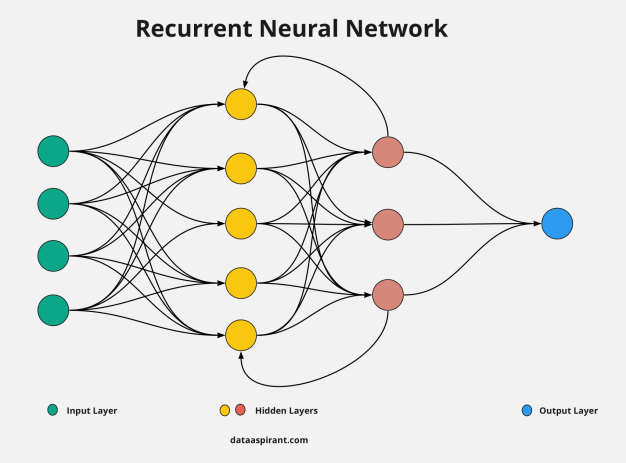
RNNs were initially developed to aid in predicting sequences; for example, the Long Short-Term Memory (LSTM) algorithm is well-known for its versatility. These networks operate exclusively on data sequences of varying lengths.
The RNN uses the previous state’s knowledge as an input value for the current prediction. As a result, it can aid in establishing short-term memory in a network, enabling the effective administration of stock price movements or other time-based data systems.
As previously stated, there are two broad categories of RNN designs that aid in issue analysis. They are as follows:
LSTMs: Effective for predicting data in temporal sequences by utilizing memory. It contains three gates: one for input, one for output, and one for forget.
Gated RNNs: Additionally, it is advantageous for data prediction of time sequences using memory. It is divided into two gates: Update and Reset.
Effective in the following situations:
One to One: A single input is coupled to a single output, as with image categorization.
One to many: A single input is connected to several output sequences, such as picture captioning, which incorporates many words from a single image.
Many to One: Sentiment Analysis is an example of a series of inputs producing a single outcome.
Many to many: As in video classification, a sequence of inputs results in outputs.
Additionally, it is widely used in language translation, dialogue modelling, and other applications.
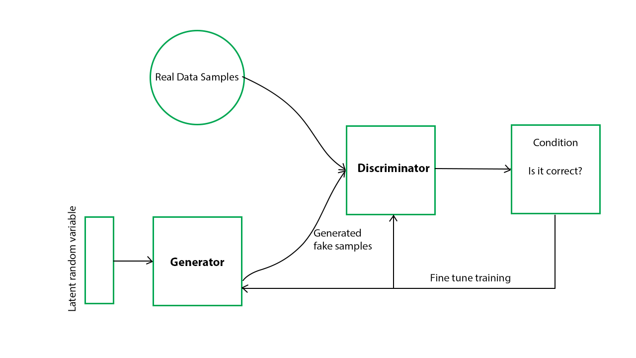
It combines a Generator and a Discriminator, two techniques for deep learning neural networks. The Discriminator aids in differentiating fictional data from real data generated by the Generator Network.
Even if the Generator continues to produce bogus data that is identical in every way, the Discriminator continues to discern real from fake. An image library might be created using simulated data generated by the Generator network in place of the original photographs. In the next step, a deconvolutional neural network would be created.
Following that, an Image Detector network would be used to determine the difference between actual and fraudulent pictures. Starting with a 50% possibility of correctness, the detector must improve its categorization quality as the generator improves its false picture synthesis. This rivalry would ultimately benefit the network’s efficacy and speed.
Effective in the following situations:
Image and Text Generation
Image Enhancement
New Drug Discovery processes
SOMs, or Self-Organizing Maps, minimize the number of random variables in a model by using unsupervised data. The output dimension is set as a two-dimensional model in this deep learning approach since each synapse links to its input and output nodes.
As each data point vies for model representation, the SOM adjusts the weights of the nearest nodes or Best Matching Units (BMUs). The weights’ values alter in response to the vicinity of a BMU. Because weights are regarded as a node feature in and of itself, the value signifies the node’s placement in the network.
Effective in the following situations:
When the datasets do not include Y-axis values.
Explorations for the dataset framework as part of the project.
AI-assisted creative initiatives in music, video, and text.
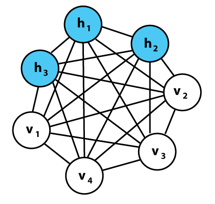
Because this network architecture lacks a fixed direction, its nodes are connected circularly. Due to the peculiarity of this approach, it is utilized to generate model parameters.
Unlike all preceding deterministic network models, the Boltzmann Machines model is stochastic in nature.
Effective in the following situations:
Monitoring of the system
Establishment of a platform for binary recommendation
Analyzing certain datasets
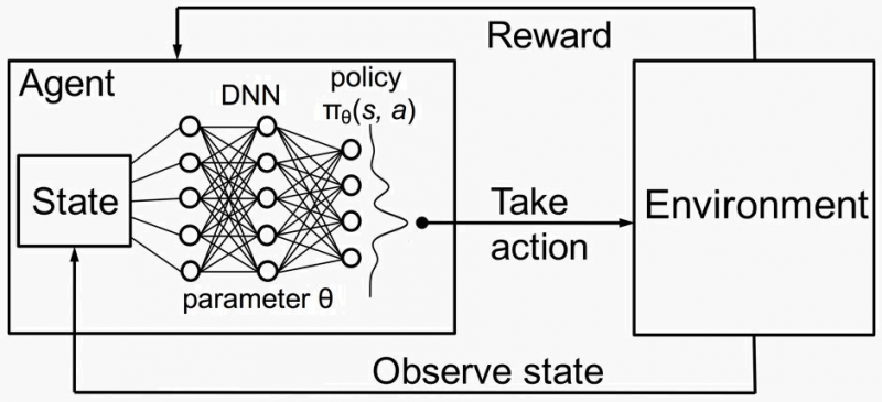
Before diving into the Deep Reinforcement Learning approach, it’s important to grasp the concept of reinforcement learning. To assist a network in achieving its goal, the agent can observe the situation and take action accordingly.
This network architecture has an input layer, an output layer, and numerous hidden multiple layers – the input layer containing the state of the environment. The model is based on repeated efforts to forecast the future reward associated with each action made in a given state of the circumstance.
Effective in the following situations:
Board Games like Chess, Poker
Self-Drive Cars
Robotics
Inventory Management
Financial tasks such as asset valuation
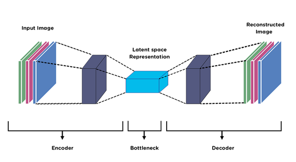
One of the most often used deep learning approaches, this model functions autonomously depending on its inputs before requiring an activation function and decoding the final output. Such a bottleneck creation results in fewer categories of data and the utilization of the majority of the inherent data structures.
Effective in the following situations:
Feature recognition
Creating an enticing recommendation model
Enhance huge datasets using characteristics
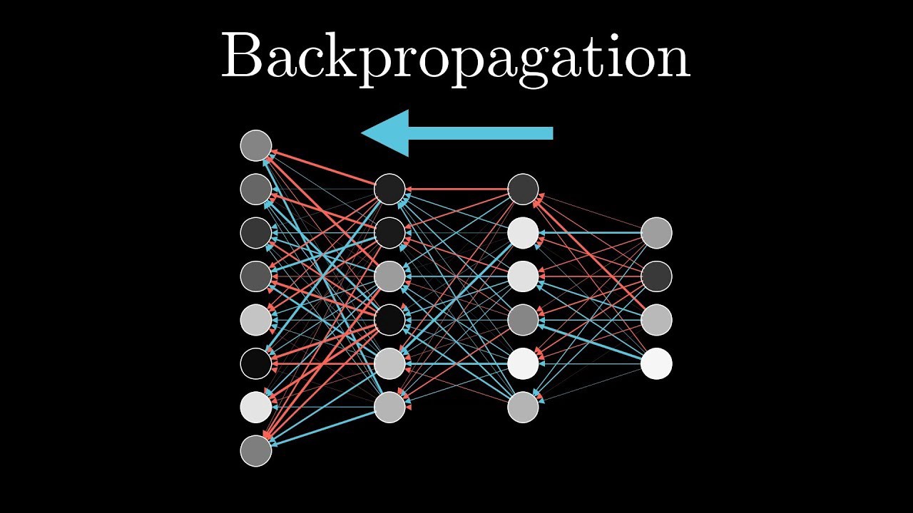
Backpropagation, or back-prop, is the basic process through which neural networks learn from data prediction mistakes in deep learning. By contrast, propagation refers to data transfer in a specific direction over a defined channel. The complete system can operate in the forward direction at the time of decision and feeds back any data indicating network deficiencies in reverse.
To begin, the network examines the parameters and decides about the data.
Second, a loss function is used to weigh it.
Thirdly, the detected fault is propagated backwards to self-correct any inaccurate parameters.
Effective in the following situations:
Data Debugging
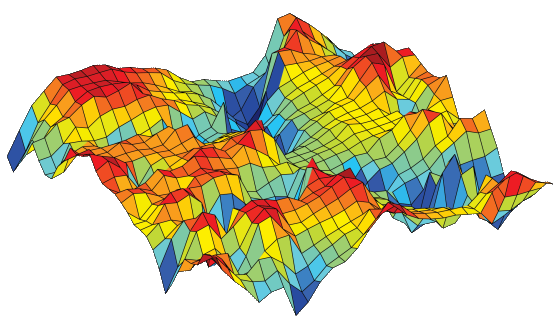
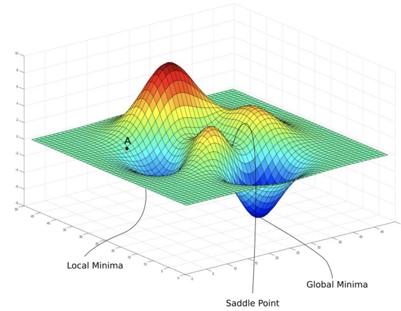
Gradient refers to a slop with a quantifiable angle and may be expressed mathematically as a relationship between variables. The link between the error produced by the neural network and the data parameters may be represented as “x” and “y” in this deep learning approach. Due to the dynamic nature of the variables in a neural network, the error can be increased or lowered with modest adjustments.
The goal of this method is to arrive at the best possible outcome. There are ways to prevent data from being caught in a neural network’s local minimum solutions, causing compilations to run slower and be less accurate.
As with the mountain’s terrain, certain functions in the neural network called Convex Functions ensure that data flows at predicted rates and reaches its smallest possible value. Due to variance in the function’s beginning values, there may be differences in the techniques through which data enters the end destination.
Effective in the following situations:
Updating parameters in a certain model
There are several techniques for deep learning approaches, each with its own set of capabilities and strategies. Once these models are found and applied to the appropriate circumstances, they can help developers achieve high-end solutions dependent on the framework they utilize. Best of luck!
Read more articles on techniques for Deep Learning on our blog!
The media shown in this article is not owned by Analytics Vidhya and are used at the Author’s discretion.
Currently, I Am pursuing my Bachelors of Technology( B.Tech) from Vellore Institute of Technology. I am very enthusiastic about programming and its real applications including software development, machine learning and data science.
Lorem ipsum dolor sit amet, consectetur adipiscing elit,