This article was published as a part of the Data Science Blogathon.

https://miro.medium.com/max/1400/1*4IGcGOqQpse_J7MMYU8dAg.png
Introduction
If you are reading this article, I am assuming that you are already familiar with Machine Learning, and have a basic idea about it. If not no worries, we will go through step by step to understand Machine Learning and Linear Regression (LR) in depth.
Table of Content
1. Introduction to Machine Learning
2. What is Regression?
3. What is Linear Regression (LR)?
4. Basic assumption of Linear Regression (LR)
5 . Implementation of Linear Regression in scikit-learn and statsmodels
Introduction to Machine Learning
Machine Learning is a part of Artificial Intelligence (AI), where the model will learn from the data and can predict the outcome. Machine Learning is a study of statistical computer algorithm that improves automatically from the data. Unlike computer algorithms, rely on human beings.
Types of Machine Learning Algorithms
Supervised Machine Learning
In Supervised Learning, we will have both the independent variable (predictors) and the dependent variable (response). Our model will be trained using both independent and dependent variables. So we can predict the outcome when the test data is given to the model. Here, using the output our model can measure its accuracy and can learn over time. In supervised learning, we will solve both Regression and Classification problems.
Unsupervised Machine Learning
In Unsupervised Learning, our model will won’t be provided an output variable to train. So we can’t use the model to predict the outcome like Supervised Learning. These algorithms will be used to analyze the data and find the hidden pattern in it. Clustering and Association Algorithms are part of unsupervised learning.
Reinforcement Learning
Reinforcement learning is the training of machine learning models which make a decision sequentially. In simple words, the output of the model will depend on the present input, and the next input will depend on the previous output of the model.
What is Regression?
Regression analysis is a statistical method that helps us to understand the relationship between dependent and one or more independent variables,
Dependent Variable
This is the Main Factor that we are trying to predict.
Independent Variable
These are the variables that have a relationship with the dependent variable.
Types of Regression Analysis
There are many types of regression analysis, but in this article, we will deal with,
1. Simple Linear Regression
2. Multiple Linear Regression
What is Linear Regression?
In Machine Learning lingo, Linear Regression (LR) means simply finding the best fitting line that explains the variability between the dependent and independent features very well or we can say it describes the linear relationship between independent and dependent features, and in linear regression, the algorithm predicts the continuous features(e.g. Salary, Price ), rather than deal with the categorical features (e.g. cat, dog).
Simple Linear Regression
Simple Linear Regression uses the slope-intercept (weight-bias) form, where our model needs to find the optimal value for both slope and intercept. So with the optimal values, the model can find the variability between the independent and dependent features and produce accurate results. In simple linear regression, the model takes a single independent and dependent variable.
There are many equations to represent a straight line, we will stick with the common equation,
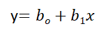
Here, y and x are the dependent variables, and independent variables respectively. b1(m) and b0(c) are slope and y-intercept respectively.
 https://d138zd1ktt9iqe.cloudfront.net/media/seo_landing_files/image-002-1602570755.png
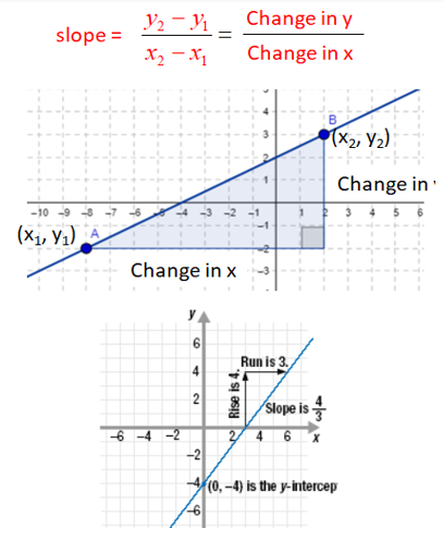
Slope(m) tells, for one unit of increase in x, How many units does it increase in y. When the line is steep, the slope will be higher, the slope will be lower for the less steep line.
Constant(c) means, What is the value of y when the x is zero.
How the Model will Select the Best Fit Line?
First, our model will try a bunch of different straight lines from that it finds the optimal line that predicts our data points well.
https://corporatefinanceinstitute.com/multiple-linear-regression
From the above picture, you can notice there are 4 lines, and any guess which will be our best fit line?
Ok, For finding the best fit line our model uses the cost function. In machine learning, every algorithm has a cost function, and in simple linear regression, the goal of our algorithm is to find a minimal value for the cost function.
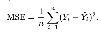
And in linear regression (LR), we have many cost functions, but mostly used cost function is MSE(Mean Squared Error). It is also known as a Least Squared Method.
https://encryptedtbn0.gstatic.com/imagesq=tbn:ANd9GcS3JnNsWSLTgU6jZiKrkWYfJ2ThDH_nL6pWw&usqp=CAU
Yi – Actual value,
Y^i – Predicted value,
n – number of records.
( yi – yi_hat ) is a Loss Function. And you can find in most times people will interchangeably use the word loss and cost function. But they are different, and we are squaring the terms to neglect the negative value.
Loss Function
It is a calculation of loss for single training data.
Cost Function
It is a calculation of average loss over the entire dataset.
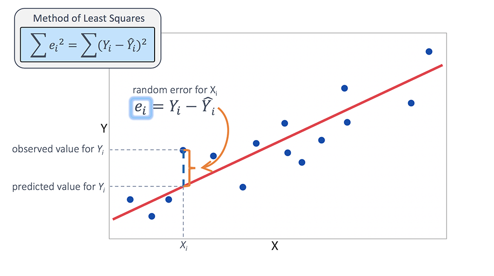
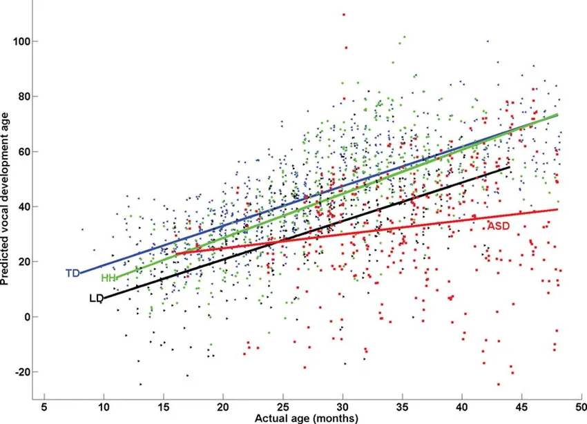
From the above picture, blue data points are representing the actual values from training data, a red line(vector) is the predicted value for that actual blue data point. we can notice a random error, the actual value-predicted value, model is trying to minimize the error between the actual and predicted value. Because in the real world we need a model, which makes the prediction very well. So our model will find the loss between all the actual and predicted values respectively. And it selects the line which has an average error of all points lower.
Steps
- Our model will fit all possible lines and find an overall average error between the actual and predicted values for each line respectively.
- Selects the line which has the lowest overall error. And that will be the best fit line.
Don’t you think our Model does a lot of Computation?
Optimization Algorithms to the recuse. We use an optimization algorithm in some machine learning algorithms and deep learning algorithms to make the computation faster. Because in machine learning the overall time complexity is important. In Linear Regression (LR) we use Gradient Descent Algorithm to find an optimal value for both slope and y-intercept. We won’t go in-depth. You can refer to some other resources to understand the Gradient Descent well.
Multiple Linear Regression
In multiple linear regression, our model will apply the same steps. In multiple linear regression instead of having a single independent variable, the model has multiple independent variables to predict the dependent variable.
![]()
where bo is the y-intercept, b1,b2,b3,b4…,bn are slopes of the independent variables x1,x2,x3,x4…,xn and y is the dependent variable.
Here instead of finding a line, our model will find the best plane in 3-Dimension, and in n-Dimension, our model will find the best hyperplane. The below diagram is for demonstration purposes.
https://aegis4048.github.io/mutiple_linear_regression_and_visualization_in_python
Assumption of Linear Regression
Linearity
The first and most obvious assumption of our model is linearity. It means, there must be a linear relationship between the dependent and independent features. Without a Linear relationship, accurate predictions won’t be possible. The most commonly used method to find the linear relationship is a correlation, Scatterplot. A correlation provides information on the strength and direction of the linear relationship between two variables.

Normality
Normality doesn’t mean our independent variable should be normally distributed. Linear Regression can work perfectly with non-normal distribution. Normality means our errors(residuals) should be normally distributed. We can get the errors of the model in the statsmodels using the below code.
errors = model.resid
We can use Histogram and statsmodels Q-Q plot to check the probability distribution of the error terms.
import scipy.stats as stats
figure = sm.graphics.qqplot(data=errors ,dist=stats.norm,
                         line='45', fit=True)
figure.show()
https://www.statsmodels.org/0.9.0/plots/graphics_gofplots_qqplot_00.png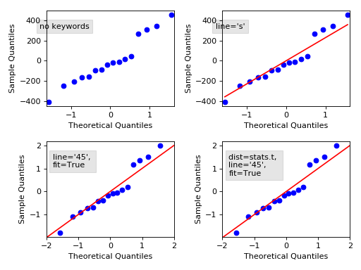
The line is drawn at 45 degrees. If there is too much deviation of the error data points from the red line, then we consider the error is not normally distributed. We also should be considered a curve at the end.
Multicollinearity
The Independent variables should not be correlated with each other, when they are correlated with each other, then we could conclude that one variable explains another variable well. So we don’t need two variables doing the same thing. eg. You have two pens, both the pens do the same which is writing so you don’t need two pens for writing (consider two pens are magical pens, so you won’t run out of ink). Before dropping one of the two variables you must also see how much does both independent variables are correlated with the dependent variable. Drop the variable which is lesser correlated. We can use many methods to find multicollinearity like vif, correlation heatmap.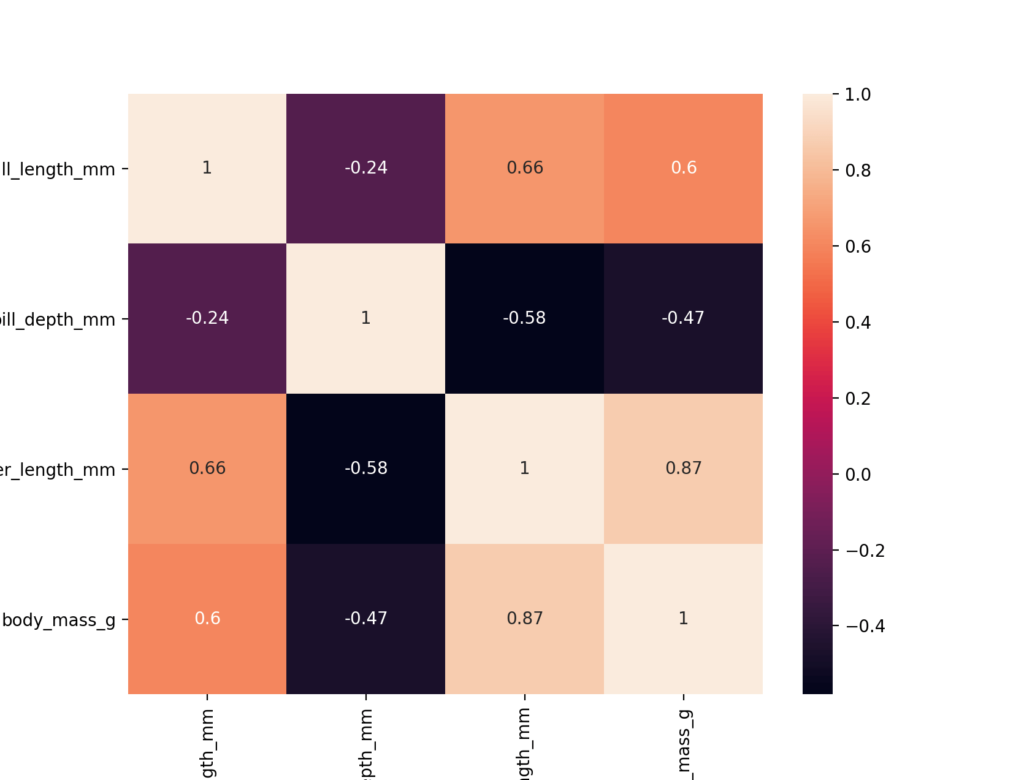
Avoid the diagonal values it is just the same features in both column and row, when we find a correlation between the same two features we will have a correlation value of 1. Here, length_mm and body_mass_g are highly correlated.
Homoscedasticity
It refers to a condition that the variance of the error(residuals) of the model should be constant for all the independent features. When we plot the errors against e independent features it should be constant over time, if not then it is considered as a Heteroscedasticity. Where the errors are not constant over time and form a funnel shape.
Implementation of Linear Regression
Let’s try to implement the linear regression in both scikit-learn and statsmodels.
| Scikit-learn | Statsmodels | |
| Intercept_ | Includes intercept_ by default | We need to add the intercept |
| Model Evaluation | The score method in scikit-learn gives us the accuracy of the model | It shows many statistical results like p-value, F-test, Confidential Interval |
| Regularization | It uses “L2” by default, We can also set the parameter to “None” if we want | It does not use any regularization parameter. |
| Advantage | It has a lot of parameters and is easy to use. | Used to infer the population parameters from sample statistics. |
Implementation of Linear Regression using sklearn,
import pandas as pd
import numpy as np
import matplotlib.pyplot as plt

# creating a dummy dataset
np.random.seed(10)
x = np.random.rand(50, 1)
y = 3 + 3 * x + np.random.rand(50, 1)

#scatterplot

plt.scatter(x,y,s=10)
plt.xlabel('x_dummy')
plt.ylabel('y_dummy')
plt.show()

#creating a model
from sklearn.linear_model import LinearRegression

# creating a object
regressor = LinearRegression()

#training the model
regressor.fit(x, y)

#using the training dataset for the prediction
pred = regressor.predict(x)

#model performance
from sklearn.metrics import r2_score, mean_squared_error
mse = mean_squared_error(y, pred)
r2 = r2_score(y, pred)#Best fit lineplt.scatter(x, y)
plt.plot(x, pred, color = 'Black', marker = 'o')

#Results
print("Mean Squared Error : ", mse)
print("R-Squared :" , r2)
print("Y-intercept :" , regressor.intercept_)
print("Slope :" , regressor.coef_)
Implementation of Linear Regression using Statsmodel,
import statsmodels.api as sm

#adding a constant
X = sm.add_constant(x)

#performing the regression
result = sm.OLS(y, x).fit()

# Result of statsmodels
print(result.summary())

                                 OLS Regression Results
=======================================================================================
Dep. Variable:                      y   R-squared (uncentered):                   0.892
Model:                            OLS   Adj. R-squared (uncentered):              0.890
Method:                 Least Squares   F-statistic:                              405.8
Date:                Wed, 09 Feb 2022   Prob (F-statistic):                    2.35e-25
Time:                        20:40:35   Log-Likelihood:                         -96.258
No. Observations:                  50   AIC:                                      194.5
Df Residuals:                      49   BIC:                                      196.4
Df Model:                           1
Covariance Type:            nonrobust
==============================================================================
                 coef    std err          t      P>|t|      [0.025      0.975]
------------------------------------------------------------------------------
x1             8.3493      0.414     20.144      0.000       7.516       9.182
==============================================================================
Omnibus:                       10.010   Durbin-Watson:                   1.850
Prob(Omnibus):                  0.007   Jarque-Bera (JB):                3.087
Skew:                           0.202   Prob(JB):                        0.214
Kurtosis:                       1.852   Cond. No.                         1.00
==============================================================================
We can see that both the models give us similar results.
Conclusion
So, having covered most of the important topics for the beginners, it is sufficient to understand, how linear regression works. If you want to dig deeper into linear regression, look at this playlist zedstatistics. For understanding, gradient descent watches these videos. For understanding the whole math behind linear regression, go through these notes. Understanding the math behind algorithms is important in Machine Learning. Happy Learning!
The media shown in this article is not owned by Analytics Vidhya and are used at the Author’s discretion.


