This article was published as a part of the Data Science Blogathon.
Introduction
Machine Learning (ML) is reaching its own and growing recognition that ML can play a crucial role in critical applications, it includes data mining, natural language processing, image recognition. ML provides all possible keys in all these fields and more, and it set us to a pillar of our future civilization.
In this post, I’ll show you step by step implementation of a Hotel Booking Cancellation predictive model using machine learning algorithms.
The data set for the implementation is https://www.kaggle.com/jessemostipak/hotel-booking-demand
This data set consists of 119,390 observations and holds booking data for a city hotel and a resort hotel in Portugal from 2015 to 2017. It has 32 variables which include reservation and arrival date, length of stay, canceled or not, the number of adults, children, or babies, the number of available parking spaces, how many special guests, companies, and agents pushed the reservation, etc.
There are many aspects considered when choosing a hotel. The main idea is to find the appropriate prediction model for predicting hotel booking cancellations which finds the finest explaining variables for customer cancellations. This Hotel Booking Cancellation model can be useful not only for the vacationer but for the hotels’ owners.
Details of Dataset
1. hotel :(H1 = Resort Hotel or H2 = City Hotel).
2. is_canceled Value: showing if the booking had been cancelled (1) or not (0).
3. lead_time: Number of days that elapsed between the entering date of the booking into the PMS and the arrival date.
4. arrival_date_year: Year of arrival date.
5. arrival_date_month: The months in which guests are coming.
6. arrival_date_week_number: Week number of year for arrival date.
7. arrival_date_day_of_month: Which day of the months guest is arriving.
8. stays_in_weekend_nights: Number of weekend stay at night (Saturday or Sunday) the guest stayed or booked to stay at the hotel.
9. stays_in_week_nights: Number of weekdays stay at night (Monday to Friday) in the hotel.
10. adults: Number of adults.
11. children: Number of children.
12. babies: Number of babies.
13. meal: Type of meal booked.
14. country: Country of origin.
15. market_segment: Through which channel hotels were booked.
16. distribution_channel: Booking distribution channel.
17. is_repeated_guest: The values indicating if the booking name was from a repeated guest (1) or not (0).
18. previous_cancellations: Show if the repeated guest has cancelled the booking before.
19. previous_bookings_not_canceled: Show if the repeated guest has not cancelled the booking before.
20. reserved_room_type: Code of room type reserved. Code is presented instead of designation for anonymity reasons.
21. assigned_room_type: Code for the type of room assigned to the booking. Code is presented instead of designation for anonymity reasons.
22. booking_changes: How many times did booking changes happen.
23. deposit_type: Indication on if the customer deposited something to confirm the booking.
24. agent: If the booking happens through agents or not.
25. company: If the booking happens through companies, the company ID that made the booking or responsible for paying the booking.
26. days_in_waiting_list: Number of days the booking was on the waiting list before the confirmation to the customer.
27. customer_type: Booking type like Transient – Transient-Party – Contract – Group.
28. adr: Average Daily Rates that described via way of means of dividing the sum of all accommodations transactions using entire numbers of staying nights.
29. required_car_parking_spaces: How many parking areas are necessary for the customers.
30. total_of_special_requests: Total unique requests from consumers.
31. reservation_status: The last status of reservation, assuming one of three categories: Canceled – booking was cancelled by the customer; Check-Out
32. reservation_status_date: The last status date.
After understanding the data, let’s implement the model.
Following are the steps for the implementation.
- Exploratory Data Analysis
- Data Pre-Processing
- Model Building
- Model Comparison
Exploratory Data Analysis on Hotel Booking Cancellation Dataset
Before you initiate data understanding or analysis or feed your data to a machine learning algorithm, the first step is to clean your data and make it in a proper form (satisfying all the conditions). It is important to understand the type of data, patterns, and correlations present in your data. Here, is the Exploratory Data Analysis comes forward, The idea of getting to know your data in depth is called Exploratory Data Analysis.
Exploratory Data Analysis is a set of techniques developed by Tukey and John Wilder in 1970. The mindset behind this is to survey and understand the data before building a model. In today’s world, Data scientists and data analysts have to go through the most time in Data Wrangling and Exploratory Data Analysis (EDA) than building the models. In the EDA, using some statistical graphs and other visualization techniques, Data Scientists and Analysts try to find different patterns, missing data, relations, outliers, and anomalies in the data. EDA helps to ask the analytical questions and visualize the answer. It varies from person to person. Commonly the questions are related to independent variables and the target variable.
Phases Involved in Exploratory Data Analysis
Data Collection
Collecting data is a starting point of exploratory data analysis. Data collection is the process of finding data from different public sites, or one can buy from private organizations and load data into our system. Kaggle and Github are familiar and known sites that provide free data.
Import Libraries
After collecting data we have to import the necessary libraries to build machine learning models. Numpy, Pandas, Matploilib, Seaborn are the known libraries used in the machine learning model.
Numpy: NumPy is a Numerical Python Library that helps perform mathematical operations.
Pandas: Panda is an open-source library that helps understand relational or labelled data.
Matplotlib: Matplotlip is a Python visualization library that helps visualize 2D array plots.
Seaborn: Seaborn is a data visualization library built on top of matplotlib.
import pandas as pd
import numpy as np
import matplotlib.pyplot as plt
import seaborn as sns
import warnings
warnings.filterwarnings('ignore')
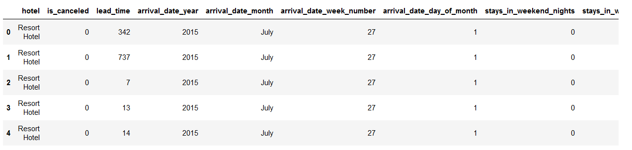
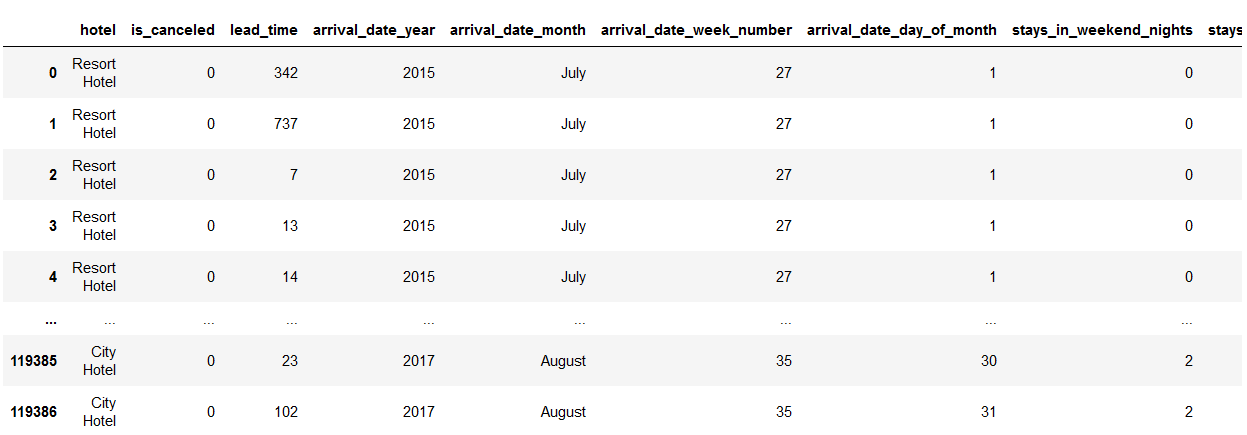
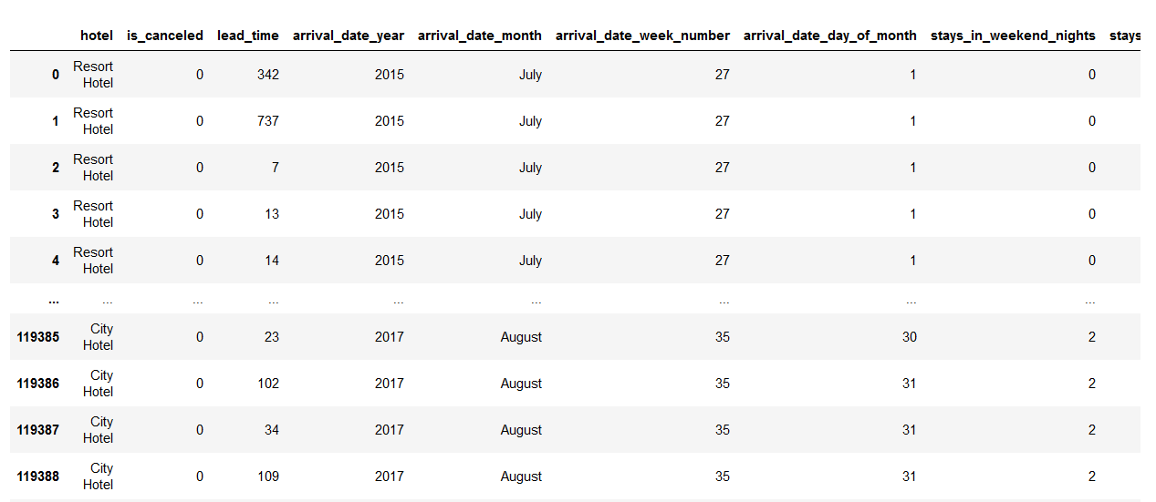
The data shown below represents the Hotel booking cancellation dataset that is available on Kaggle.
#Read and load data
df = pd.read_csv("hotel_bookings.csv")
#Display data
df.head()
Data Cleaning
Real-world raw data is often incomplete, inconsistent, and lacking in certain behaviors or trends. The raw data contain many errors. So, once collected, the next step machine learning pipeline is to clean data which refers to removing unwanted data.
Some steps which are used to clean data are:
- Remove missing values, outliers, and unnecessary rows/ columns.
- Check and impute null values.
- Check Imbalanced data.
- Re-indexing and reformatting our data.
Let’s clean our Hotel booking cancellation dataset.
First, have to check if our data holds duplicate values.
Pandas duplicated() method helps to return duplicate values only, and any() method returns a boolean series that is True only if the conditions are true.
#Check if data holds duplicate values.
df.duplicated().any()

Dataset holds the duplicate entries.
Pandas drop_duplicate() method helps to remove duplicate entries.
The keep parameter is set to False so that only Unique values are taken and the duplicate values are removed from the data.
#Drop Duplicate entries
df.drop_duplicates(inplace= False)# will keep first row and others consider as duplicate
Now check the number of missing values in each column and the percentage of missing values in columns. Pandas isna() method helps to find out null values.
null =100 *(df.isna().sum() /df.shape[0])
null
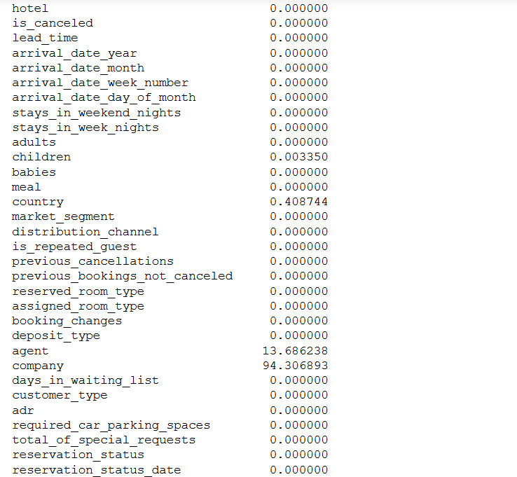
Column company holds 94% missing data, so we can drop that column.
df.drop('company',axis=1, inplace = True)
Let’s impute the missing values.
Before imputing missing values, it is necessary to understand the reason and relationship of missing data with columns. Missing data can be MAR, MCAR, and MNAR.
- MCAR (Missing completely at random): The values in the missing column are randomly missing and do not depend on the other column values.
- MAR (Missing at random): The values in the missing column are dependent on some additional features.
- MNAR (Missing not at random): The data is not missing randomly there might be some reason behind that.
To understand missing values in-depth refer to this link https://www.analyticsvidhya.com/blog/2021/10/how-to-deal-with-missing-data-using-python/
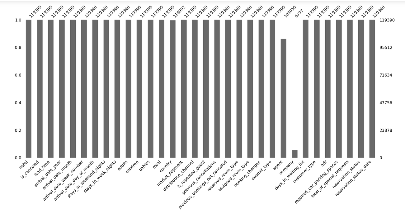
import missingno as msno
msno.bar(df)
plt.show()
msno.heatmap(df)
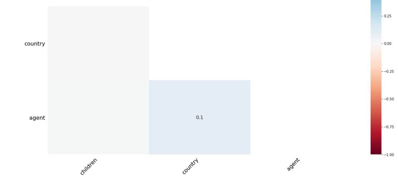
There is a 1% relationship between the agent and the company. So that we can impute missing values easily.
df.fillna(0, inplace = True)
Check dataset is a balanced dataset or not.
To understand the balanced and imbalanced dataset, Let’s take a simple example if in our data set we have equal numbers or approximately the same number of positive and negative values then we can say our dataset is in balance. If there is a high difference in both positive and negative values then the dataset is an imbalanced dataset.
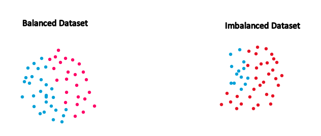
In such a case classifiers tend to make biased learning model that has a more inferior predictive accuracy over the minority classes compared to the majority classes.
Methods that Help to Handle Imbalanced Datasets
Evaluation Matrix
select the right evaluation matrix that is robust to the imbalanced dataset such as confusion matrix, f1 score, precision, Recall.
A simple and yet good metric that always helps when dealing with classification problems is the confusion matrix. A confusion matrix is a table that is used to represent the performance of a classification model (or “classifier”) on a set of test data for which the true values are known. Thus, it is a terrific starting point for any classification model evaluation.
The following graphic model helps to summarize the metrics derived from the confusion matrix.
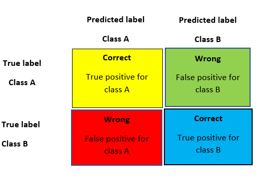
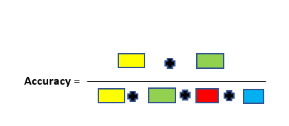
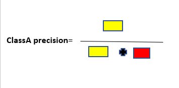
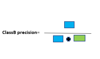
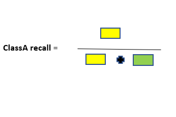
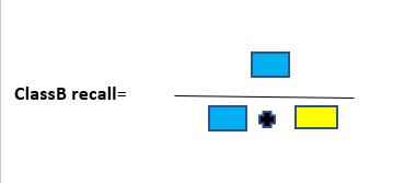
To the quick description of these metrics. The accuracy of the model is fundamentally the total number of correct predictions divided by a total number of predictions. The precision of a class defines how trust-able is the outcome is when the model answers that a point belongs to that class. The recall of a class represents how nicely the model is able to detect that class. The F1 score of a class is given by the harmonic mean of precision and recall (2×precision×recall / (precision + recall)), it combines precision and recall of a class in one metric.
For a given class, the different combinations of recall and precision have the following meanings :
- high recall + high precision: the class is completely handled by the model
- low recall + high precision: the model can’t detect the class well but is positively trust-able when it does
- high recall + low precision: the class is well detected but the model also contains points of other classes in it
- low recall + low precision: the class is wrongly handled by the model.
Random resampling Technique
One approach to addressing the imbalanced dataset problem is to randomly resample the training dataset. Two main approaches that come under the random resample are undersampling and oversampling.
Under-sampling reduces the number of majority samples to balance the class distribution. Since it is removing observations from the original data set there is a high chance of discarding data. Over-sampling boosts the number of minority class members in the training set. The benefit of over-sampling is that no information from the original training set is lost, as all observations from the minority and majority classes are kept which leads to overfitting.
SMOTE
It helps to overcome the disadvantage of oversampling. The advantage of SMOTE is that you are not generating duplicates but rather creating synthetic data points that are slightly different from the original data.
df['is_canceled'].value_counts()
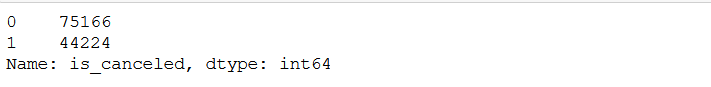
Our dataset has an imbalanced dataset.
Handling Outliers
There are two types of outliers:
- Univariate outliers: Outliers are the data points that are away from the expected range of values. In Univariate analysis single variable is considered to detect outliers.
- Multivariate outliers: These outliers are dependent on the correlation between two variables.
Univariate Analysis
In the univariate analysis, we consider only a single variable that can be numerical or categorical. For numerical continue variables, we can use a histogram or scatter plot, and for categorical data, we commonly preferred bar plots or pie charts.
Bivariate Analysis
We can handle bivariate analysis in 3 ways:
Numeric and Numeric:
In Numeric-Numeric analysis, we compare both numeric variables. The scatter plots, pair plots, and correlation matrics compare two numeric columns.
Scatter Plot
A scatter plot represents every data point in the graph format. It shows the relationship of two data means how the values from one column fluctuate according to the corresponding values in another column.
Pair Plot
Pair plots compare multiple variables at the same time. Pair plots save spaces and compare various variables at the same time.
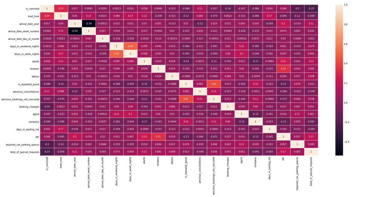
Correlation Matrix
A correlation matrix glimpses the correlation between different variables. The correlation between two variables is determined by the correlation coefficient.
Numeric – Categorical Analysis
In numeric-categorical analysis, one variable is a numeric type and the other is a categorical variable. We can use group by function or box plot to perform numeric-categorical analysis.
Categorical-categorical Analysis
The chi-square test determines the association between categorical variables. The Chi-square test calculates based on the difference between expected frequencies and the observed frequencies in one or more categories of the frequency table.
The Zero probability indicates a complete dependency between two categorical variables. The One probability indicates two categorical variables are completely independent.
Data Preprocessing and Analysis
babies, adults, and children can not be zero at the same time, so we will drop all the observations having zero at the same time.
filter = (df.children == 0) & (df.adults == 0) & (df.babies == 0)
df[filter]
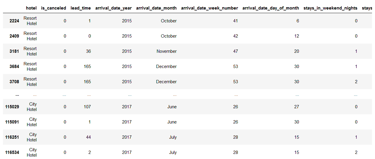
df = df[~filter]
df
After dropping…..
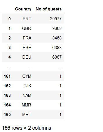
From where the most guest are coming?
guest_city = df[df['is_canceled'] == 0]['country'].value_counts().reset_index()
guest_city.columns = ['Country', 'No of guests']
guest_city
Let’s visualized using graphics visualization
import folium
from folium.plugins import HeatMap
import plotly.express as px
basemap = folium.Map()
guests_map = px.choropleth(guest_city, locations = guest_city['Country'],
                           color = guest_city['No of guests'], hover_name = guest_city['Country'])
guests_map.show()
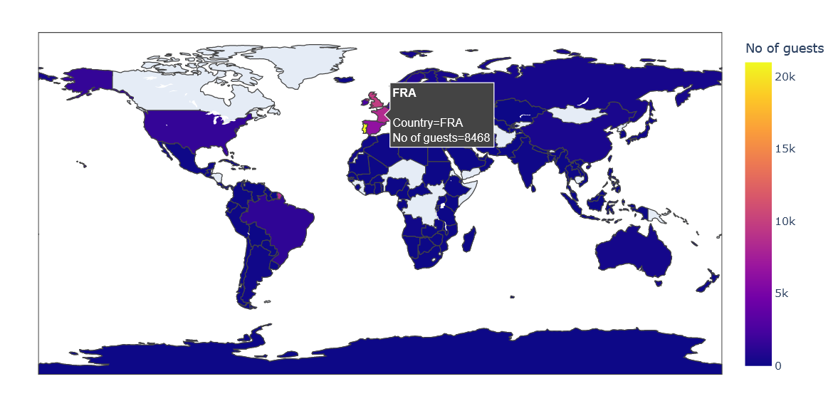
Most guests are from Portugal and other countries in Europe.
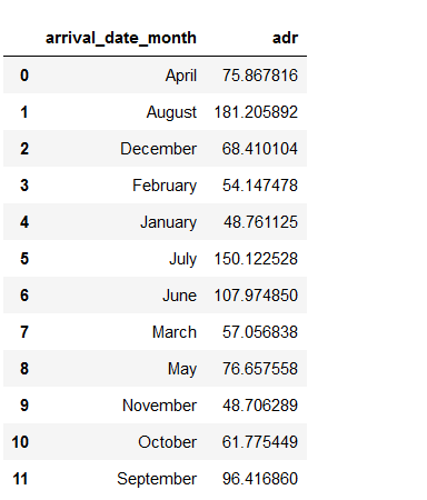
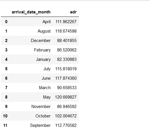
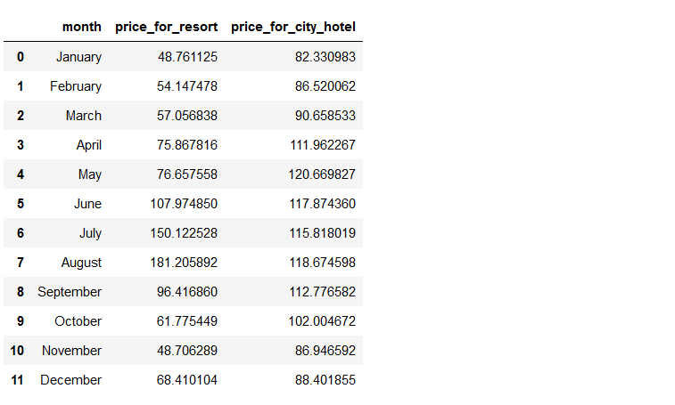
What are the Room prices overnights for each month?
data_resort = df[(df['hotel'] == 'Resort Hotel') & (df['is_canceled'] == 0)]
data_city = df[(df['hotel'] == 'City Hotel') & (df['is_canceled'] == 0)]_canceled'] == 0)]
resort_hotel = data_resort.groupby(['arrival_date_month'])['adr'].mean().reset_index()
resort_hotel
city_hotel=data_city.groupby(['arrival_date_month'])['adr'].mean().reset_index()
city_hotel
Now we observe here that the month column is not in order, and if we visualize we will get improper conclusions.
So, first, we have to provide the right hierarchy to the month column.
Now we observe here that the month column is not in order, and if we visualize we will get improper conclusions.
So, first, we have to provide the right hierarchy to the month column.
!pip install sort-dataframeby-monthorweek
!pip install sorted-months-weekdays
import sort_dataframeby_monthorweek as sd
def sort_month(df, column_name):
    return sd.Sort_Dataframeby_Month(df, column_name)
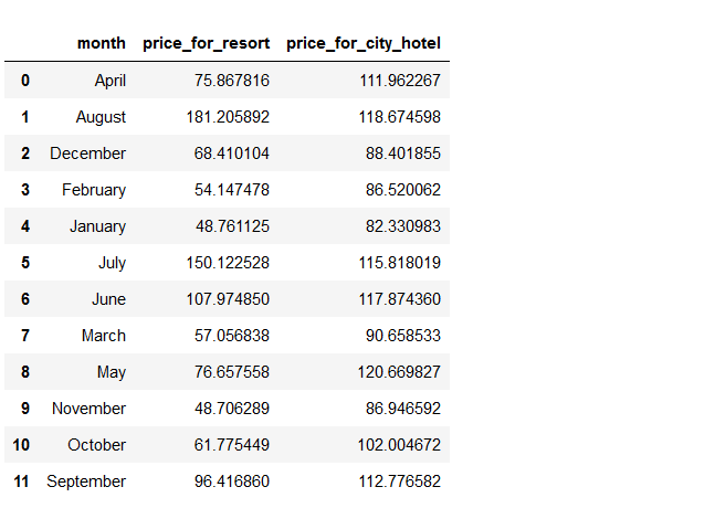
final_prices = sort_month(final_hotel, 'month')
final_prices
Let’s visualize by graphics
plt.figure(figsize = (17, 8))
px.line(final_prices, x = 'month', y = ['price_for_resort','price_for_city_hotel'],
        title = 'Room price per night over the Months', template = 'plotly_dark')
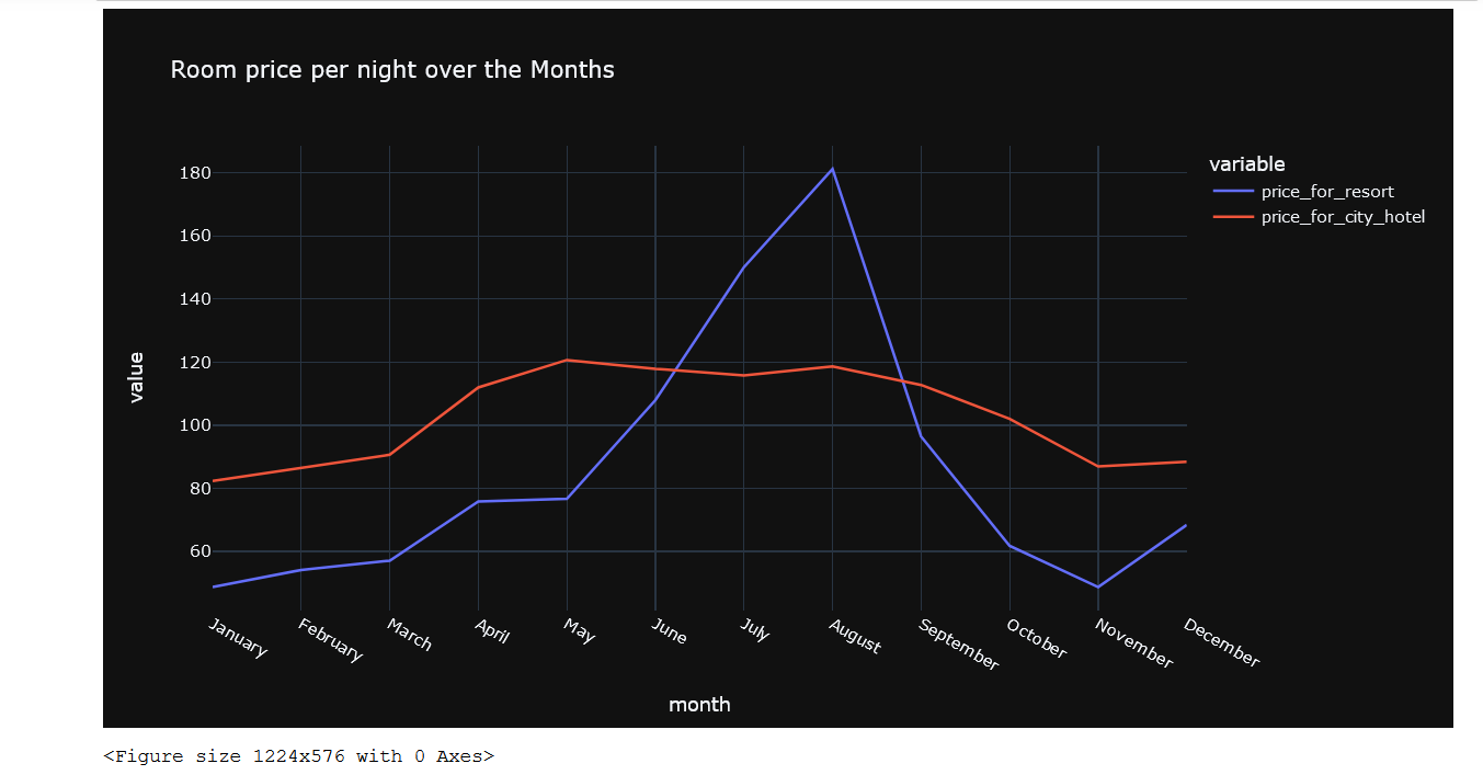
This plot clearly shows that prices in the Resort Hotel are much higher during the summer
plt.<a onclick="parent.postMessage({'referent':'.matplotlib.pyplot.figure'}, '*')">figure(figsize = (24, 12))

corr = df.corr()
sns.<a onclick="parent.postMessage({'referent':'.seaborn.heatmap'}, '*')">heatmap(corr, annot = True, linewidths = 1)
plt.<a onclick="parent.postMessage({'referent':'.matplotlib.pyplot.show'}, '*')">show()
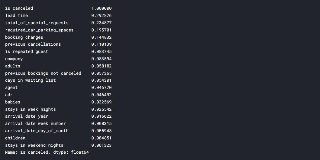
correlation = df.corr()['is_canceled'].abs().sort_values(ascending = False)
correlation
# dropping columns that are not useful

useless_col = ['days_in_waiting_list', 'arrival_date_year', 'arrival_date_year', 'assigned_room_type', 'booking_changes',
               'reservation_status', 'country', 'days_in_waiting_list']

df.drop(useless_col, axis = 1, inplace = True)
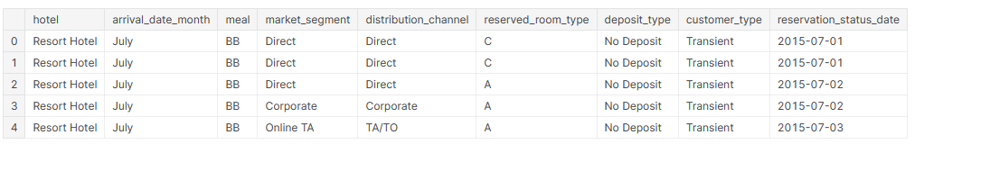
cat_cols = [<a onclick="parent.postMessage({'referent':'.kaggle.usercode.17158237.65503949.[4969,4972].col'}, '*')">col for <a onclick="parent.postMessage({'referent':'.kaggle.usercode.17158237.65503949.[4969,4972].col'}, '*')">col in df.columns if df[<a onclick="parent.postMessage({'referent':'.kaggle.usercode.17158237.65503949.[4969,4972].col'}, '*')">col].dtype == 'O']
cat_cols
cat_df = df[cat_cols]
cat_df.head()
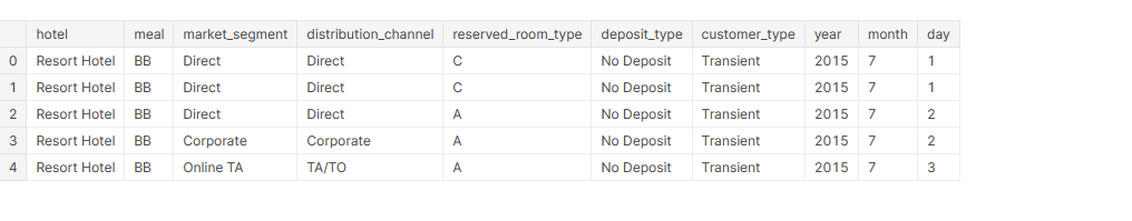
cat_df['reservation_status_date'] = pd.<a onclick="parent.postMessage({'referent':'.pandas.to_datetime'}, '*')">to_datetime(cat_df['reservation_status_date'])

cat_df['year'] = cat_df['reservation_status_date'].dt.year
cat_df['month'] = cat_df['reservation_status_date'].dt.month
cat_df['day'] = cat_df['reservation_status_date'].dt.day
cat_df.drop(['reservation_status_date','arrival_date_month'] , axis = 1, inplace = True)
cat_df.head()
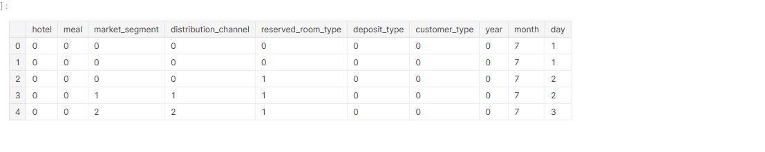
# encoding categorical variables

cat_df['hotel'] = cat_df['hotel'].map({'Resort Hotel' : 0, 'City Hotel' : 1})

cat_df['meal'] = cat_df['meal'].map({'BB' : 0, 'FB': 1, 'HB': 2, 'SC': 3, 'Undefined': 4})

cat_df['market_segment'] = cat_df['market_segment'].map({'Direct': 0, 'Corporate': 1, 'Online TA': 2, 'Offline TA/TO': 3,
                                                           'Complementary': 4, 'Groups': 5, 'Undefined': 6, 'Aviation': 7})

cat_df['distribution_channel'] = cat_df['distribution_channel'].map({'Direct': 0, 'Corporate': 1, 'TA/TO': 2, 'Undefined': 3,
                                                                       'GDS': 4})

cat_df['reserved_room_type'] = cat_df['reserved_room_type'].map({'C': 0, 'A': 1, 'D': 2, 'E': 3, 'G': 4, 'F': 5, 'H': 6,
                                                                   'L': 7, 'B': 8})

cat_df['deposit_type'] = cat_df['deposit_type'].map({'No Deposit': 0, 'Refundable': 1, 'Non Refund': 3})

cat_df['customer_type'] = cat_df['customer_type'].map({'Transient': 0, 'Contract': 1, 'Transient-Party': 2, 'Group': 3})

cat_df['year'] = cat_df['year'].map({2015: 0, 2014: 1, 2016: 2, 2017: 3})
cat_df.head()
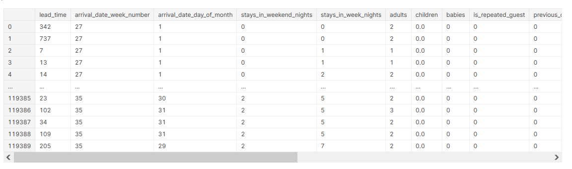
num_df = df.drop(columns = cat_cols, axis = 1)
num_df.drop('is_canceled', axis = 1, inplace = True)
num_df
num_df.var()
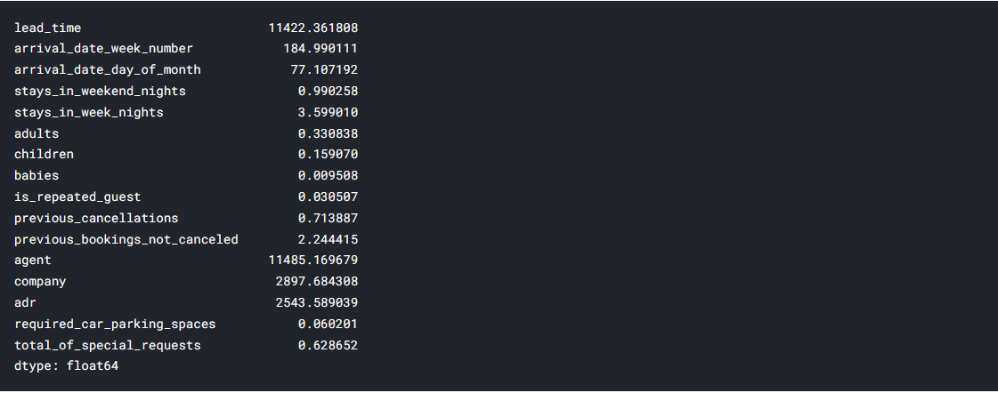
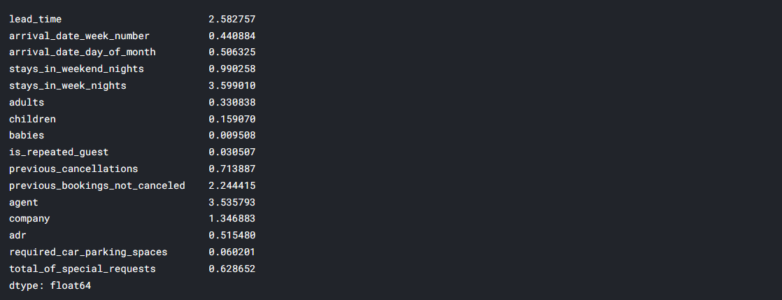
Normalized numerical columns that have high variance
num_df['lead_time'] = np.<a onclick="parent.postMessage({'referent':'.numpy.log'}, '*')">log(num_df['lead_time'] + 1)
num_df['arrival_date_week_number'] = np.<a onclick="parent.postMessage({'referent':'.numpy.log'}, '*')">log(num_df['arrival_date_week_number'] + 1)
num_df['arrival_date_day_of_month'] = np.<a onclick="parent.postMessage({'referent':'.numpy.log'}, '*')">log(num_df['arrival_date_day_of_month'] + 1)
num_df['agent'] = np.<a onclick="parent.postMessage({'referent':'.numpy.log'}, '*')">log(num_df['agent'] + 1)
num_df['company'] = np.<a onclick="parent.postMessage({'referent':'.numpy.log'}, '*')">log(num_df['company'] + 1)
num_df['adr'] = np.<a onclick="parent.postMessage({'referent':'.numpy.log'}, '*')">log(num_df['adr'] + 1)
Model Building
from sklearn.model_selection import train_test_split, GridSearchCV
from sklearn.preprocessing import StandardScaler
from sklearn.metrics import accuracy_score, confusion_matrix, classification_report
from sklearn.linear_model import LogisticRegression
from sklearn.neighbors import KNeighborsClassifier
from sklearn.svm import SVC
from sklearn.tree import DecisionTreeClassifier
from sklearn.ensemble import RandomForestClassifier
from sklearn.ensemble import RandomForestClassifier
X = pd.<a onclick="parent.postMessage({'referent':'.pandas.concat'}, '*')">concat([cat_df, num_df], axis = 1)
y = df['is_canceled']
X_train, X_test, y_train, y_test = train_test_split(X, y, test_size = 0.30)
Logistic Regression
Logistic regression comes under the most popular Supervised Machine Learning algorithms. Logistic regression predicts the categorical dependent variable using a given set of independent variables. The categorical dependent variable should be either Yes or No, 0 or 1, true or false, etc. Logistic regression is much comparable to Linear Regression only implementation is different. Linear Regression solves the Regression problems, and Logistic regression is used for solving the classification problems. Instead of fitting the regression line, In logistic regression, we fit the sigmoid S function, which predicts two maximum values(0,1). The curve from the logistic function indicates the likelihood of something such as whether rain comes or not based on weather conditions.
Logistic Function (Sigmoid Function)
To map the predicted values to probabilities sigmoid function is used. It maps the values between the range of 0 and 1. The threshold value is used in the logistic regression to compute the S Shape. The threshold value defines the probability of either 0 or 1. The value above the threshold tends to be 1, and the values below the threshold tend to 0.
Assumptions for Logistic Regression
- The data must follow a normal distribution.
- The dependent variable must be categorical.
- The independent variable should not have multi-collinearity
Type of Logistic Regression
The Logistic regression is classified into three types based on the categories.
- Binomial: If dependent variables hold two categories such as 0 or 1, male or female, pass or fail, it comes into binomial logistic regression.
- Multinomial: If a dependent variable holds three or more possible unordered categorical variables, such as cat, dog, lion, it comes into multinomial logistic regression.
- Ordinal: If the dependent variable holds three or more possible ordered categorical variables such as low, medium, high, it comes into ordinal logistic regression.
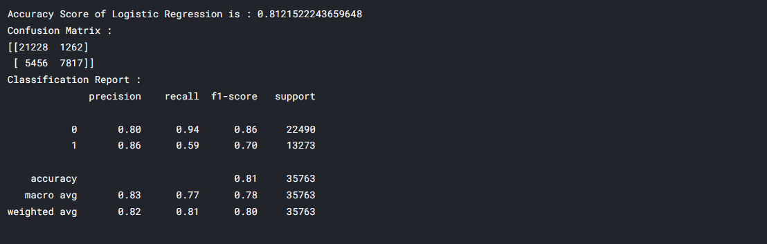
lr = LogisticRegression()
lr.fit(X_train, y_train)

y_pred_lr = lr.predict(X_test)

acc_lr = accuracy_score(y_test, y_pred_lr)
conf = confusion_matrix(y_test, y_pred_lr)
clf_report = classification_report(y_test, y_pred_lr)

print(f"Accuracy Score of Logistic Regression is : {acc_lr}")
print(f"Confusion Matrix : n{conf}")
print(f"Classification Report : n{clf_report}")
Applying KNN Algorithm on Hotel Booking Cancellation Dataset
K-Nearest Neighbor is another effortless supervised Machine Learning algorithm. KNN algorithm assumes the similarities between new data and available data. K-NN algorithm stores all the available data and classifies a new data point based on the similarity. KNN is used to solve both classification and regression problems. K-NN is a non-parametric algorithm, which means it does not make any assumptions on underlying data. KNN is a lazy learner algorithm because the KNN algorithm stores the dataset during the training phase. When KNN gets new data, then it classifies that data into a category that is much similar to the new data. Example: Suppose, we have an image of an animal that looks like a cat and a dog, but we want to understand whether it is a cat or a dog. Using the KNN algorithm we can perform this identification, as it works on similarity dimensions. Our KNN model will find the similar features of the new data set to the cats and dogs images, and based on the most similar features it will put it in either the cat or dog category. To find the nearest value we use the Euclidean distance.
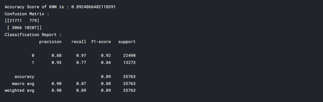
knn = KNeighborsClassifier()
knn.fit(X_train, y_train)

y_pred_knn = knn.predict(X_test)

acc_knn = accuracy_score(y_test, y_pred_knn)
conf = confusion_matrix(y_test, y_pred_knn)
clf_report = classification_report(y_test, y_pred_knn)

print(f"Accuracy Score of KNN is : {acc_knn}")
print(f"Confusion Matrix : n{conf}")
print(f"Classification Report : n{clf_report}")
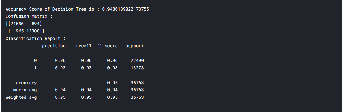
Decision Tree Classification Algorithm
The Decision Tree algorithm belongs to the family of non-parametric, supervised learning algorithms. It allows for solving regression and classification problems too.
dtc = DecisionTreeClassifier()
dtc.fit(X_train, y_train)

y_pred_dtc = dtc.predict(X_test)

acc_dtc = accuracy_score(y_test, y_pred_dtc)
conf = confusion_matrix(y_test, y_pred_dtc)
clf_report = classification_report(y_test, y_pred_dtc)

print(f"Accuracy Score of Decision Tree is : {acc_dtc}")
print(f"Confusion Matrix : n{conf}")
print(f"Classification Report : n{clf_report}")
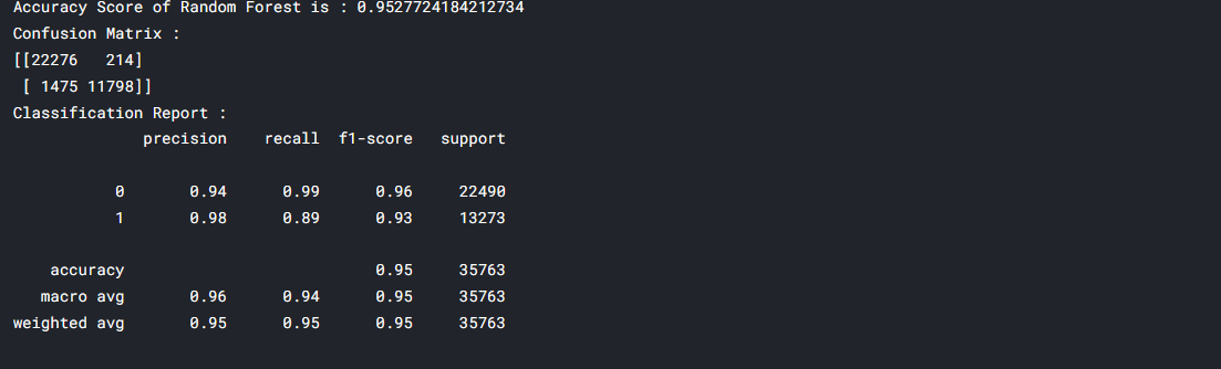
Random Forest Algorithm
Random Forest is a popular supervised machine learning algorithm. The random forest algorithm implements both Classification and Regression problems in ML. The Random Forest is a classifier that includes several decision trees instead of relying on one decision tree, the random forest takes the prediction from each tree, and based on the majority votes of predictions, it predicts the final output. The greater number of trees in the forest leads to higher accuracy and prevents the problem of overfitting.
rd_clf = RandomForestClassifier()
rd_clf.fit(X_train, y_train)

y_pred_rd_clf = rd_clf.predict(X_test)

acc_rd_clf = accuracy_score(y_test, y_pred_rd_clf)
conf = confusion_matrix(y_test, y_pred_rd_clf)
clf_report = classification_report(y_test, y_pred_rd_clf)

print(f"Accuracy Score of Random Forest is : {acc_rd_clf}")
print(f"Confusion Matrix : n{conf}")
print(f"Classification Report : n{clf_report}")
Summary
The given dataset is a supervised classification dataset. It holds booking information for a city hotel and a resort hotel with information such as How and when the booking was made, the length of passengers’ stay with the number of parking slots available, the number of adults, children, and babies. The Logistic regression, K-Nearest Neighbor, Decision Tree, Random Forest algorithms are used to handle this supervised classification model. Among these four machine learning algorithms, Random forest and Decision trees perform well with respect to accuracy.
I hope this article helps you to build your machine learning model.
The media shown in this article is not owned by Analytics Vidhya and are used at the Author’s discretion.


interesting post, thanks for sharing.
final_hotel is not defined any shere can u please check these and reply as soon as possible So, first, we have to provide the right hierarchy to the month column. !pip install sort-dataframeby-monthorweek !pip install sorted-months-weekdays import sort_dataframeby_monthorweek as sd def sort_month(df, column_name): return sd.Sort_Dataframeby_Month(df, column_name) final_prices = sort_month(final_hotel, 'month') final_prices
Merge resort_hotel and city_hotel, and rename the columns. final_hotel = pd.merge(resort_hotel, city_hotel, on="arrival_date_month", suffixes=('_for_resort', '_for_city')) final_hotel.rename(columns={'arrival_date_month': 'month', 'adr_for_resort': 'price_for_resort', 'adr_for_city': 'price_for_city_hotel'}, inplace=True)