Introduction to DenseNets (Dense CNN)
Introduction
Here we’re going to summarize a convolutional-network architecture called densely-connected-convolutional networks or DenseNet architecture. So the problem that they’re trying to solve with the density of architecture is to increase the depth of the convolutional neural network.
Here we first learn about what is a dense net and why this is useful and then we go with a coding part.
This article was published as a part of the Data Science Blogathon.
Table of contents
What are DenseNets?
So we all know about a CNN (convolutional neural network) which is useful for image classification. more about CNN.
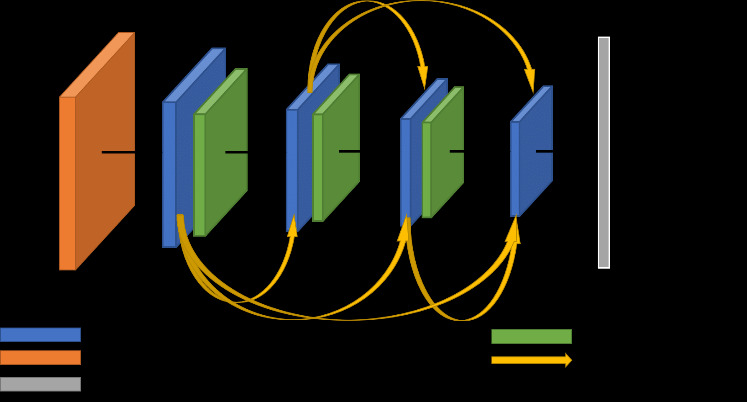
So dense net is densely connected-convolutional networks. It is very similar to a ResNet with some-fundamental differences. ResNet is using an additive method that means they take a previous output as an input for a future layer, & in DenseNet takes all previous output as an input for a future layer as shown in the above image.
Why do we need DenseNets?
So DenseNet architecture was specially developed to improve accuracy caused by the vanishing gradient in high-level neural networks due to the long distance between input and output layers & the information vanishes before reaching its destination.
DenseNet Architecture VS ResNet Architecture.
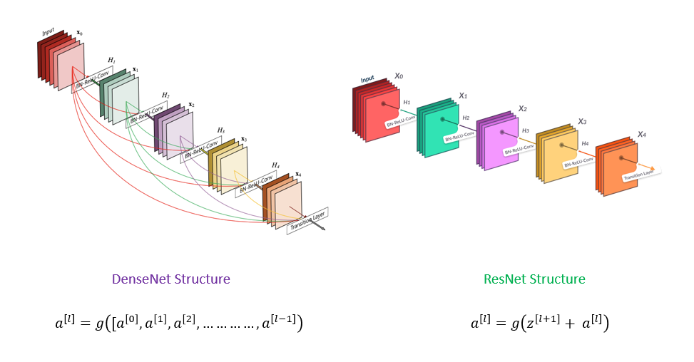
Source: paperswithcode
So suppose we have a capital L number of layers, In a typical network with L layers, there will be L
connections, that is, connections between the layers. However, in a DenseNet architecture, there will be about L
and L plus one by two connections L(L+1)/2. So in a dense net, we have less number of layers than the other model, so here we can train more than 100 layers of the model very easily by using this technique.
DenseBlocks And Layers
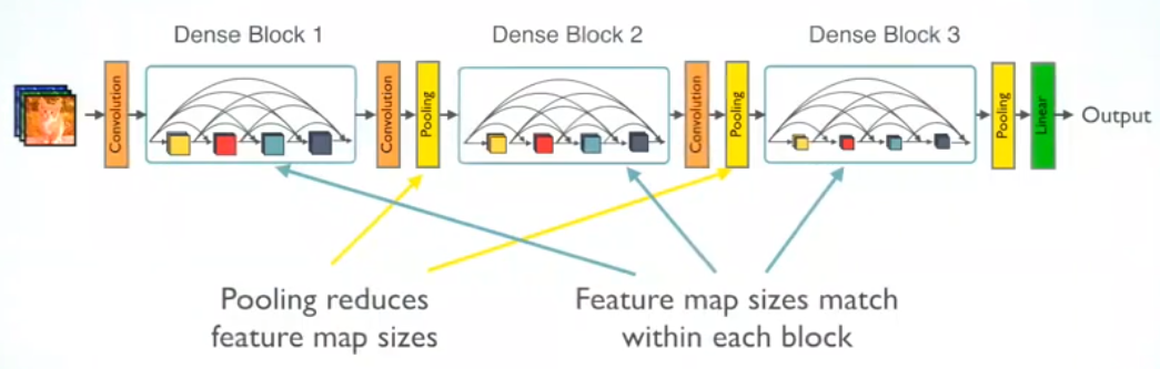
Source: Towards Data Science
Here as we go deeper into the network this becomes a kind of unsustainable, if you go 2nd layer to 3rd layer so 3rd layer takes an input not only 2nd layer but it takes input all previous layers.
So let’s say we have about ten layers. Then the 10th layer will take us to input all the feature maps from the preceding nine layers. Now, if each of these layers, let’s produce 128 feature
maps and there is a feature map explosion. to overcome this problem we create a dense block here and So each dense block contains a prespecified number of layers inside them.
and the output from that particular dense block is given to what is called a transition layer and this layer is like one by one convolution followed by Max pooling to reduce the size of
the feature maps. So the transition layer allows for Max pooling, which typically leads to a reduction in the size of your feature maps.
As a given fig, we can see two blocks first one is the convolution layer and the second is the pooling layer, and combinations of both are the transition layer.
So following some Advantages of the dense net.
- Parameter efficiency – Every layer adds only a limited number of parameters- for e.g. only about 12 kernels are learned per layer
- Implicit deep supervision – Improved flow of gradient through the network- Feature maps in all layers have direct access to the loss function and its gradient.
Important concept in DenseNet
- Growth rate – This
determines the number of feature maps output into individual layers inside dense blocks. - Dense connectivity – By dense connectivity, we mean that within a dense block each layer gets us input
feature maps from the previous layer as seen in this figure. - Composite functions – So the sequence of operations inside a layer goes as follows. So we have batch normalization, followed by an application of Relu, and then a convolution layer (that will be one
convolution layer) - Transition layers – The transition layers aggregate the feature maps from a dense block and reduce its
dimensions. So Max Pooling is enabled here.
So till this, we got a basic idea about what is a dense net, and how it internally works. So we take a simple example and understand the code here.
DenseNets On CIFAR-10
Here we apply a DenseNet on the CIFAR-10 dataset, The CIFAR-10 dataset consists of 60000 32×32 colour images in 10 classes, with 6000 images per class. There are 50000 training images and 10000 test images and more about CIFAR-10 click here.
So the 10 classes are as follows:-
| airplane |  |  |  |  |  |  |  |  |  |  |
| automobile |  |  |  |  |  |  |  |  |  |  |
| bird |  |  |  |  |  |  |  |  |  |  |
| cat |  |  |  |  |  |  |  |  |  |  |
| deer |  |  |  |  |  |  |  |  |  |  |
| dog |  |  |  |  |  |  |  |  |  |  |
| frog |  |  |  |  |  |  |  |  |  |  |
| horse |  |  |  |  |  |  |  |  |  |  |
| ship |  |  |  |  |  |  |  |  |  |  |
| truck |  |  |  |  |  |  |  |  |  |  |
Images credit – https://www.cs.toronto.edu/~kriz/cifar.html
So first we load the dataset using a Keras library and then we do one-hot encoding for the or all classes.
# Load CIFAR10 Data
(X_train, y_train), (X_test, y_test) = tf.keras.datasets.cifar10.load_data()
image_height, image_width, channel_size = X_train.shape[1],X_train.shape[2],X_train.shape[3]
# convert to one hot encoing
y_train = tf.keras.utils.to_categorical(y_train, num_classes)
y_test = tf.keras.utils.to_categorical(y_test, num_classes)
X_train.shape, X_test.shape
((50000, 32, 32, 3), (10000, 32, 32, 3))All data is in array format so first, we normalize the data by dividing a 255.0 and here we take a 255.0 because our data is RGB so we know all RGB pixels values lie between 0 to 255.
X_train = X_train / 255.0
X_test = X_test / 255.0
Now we Build DenseNet as follows-
def denseblock(input, num_filter = 12, dropout_rate = 0.2):
    global compression
    temp = input
    for _ in range(l):
        BatchNorm = layers.BatchNormalization()(temp)
        relu = layers.Activation('relu')(BatchNorm)
        Conv2D_3_3 = layers.Conv2D(int(num_filter*compression), (3,3), use_bias=False ,padding='same')(relu)
        if dropout_rate>0:
            Conv2D_3_3 = layers.Dropout(dropout_rate)(Conv2D_3_3)
        concat = layers.Concatenate(axis=-1)([temp,Conv2D_3_3])
        temp = concat
    return temp
## transition Blosck
def transition(input, num_filter = 12, dropout_rate = 0.2):
    global compression
    BatchNorm = layers.BatchNormalization()(input)
    relu = layers.Activation('relu')(BatchNorm)
    Conv2D_BottleNeck = layers.Conv2D(int(num_filter*compression), (1,1), use_bias=False ,padding='same')(relu)
    if dropout_rate>0:
         Conv2D_BottleNeck = layers.Dropout(dropout_rate)(Conv2D_BottleNeck)
    avg = layers.AveragePooling2D(pool_size=(2,2))(Conv2D_BottleNeck)
    return avg
#output layer
def output_layer(input):
    global compression
    BatchNorm = layers.BatchNormalization()(input)
    relu = layers.Activation('relu')(BatchNorm)
    AvgPooling = layers.AveragePooling2D(pool_size=(2,2))(relu)
    flat = layers.Flatten()(AvgPooling)
    output = layers.Dense(num_classes, activation='softmax')(flat)
    return output
Now we create a model with the two DenseNet blocks-
l = 7
input = layers.Input(shape=(image_height, image_width, channel_size,))
First_Conv2D = layers.Conv2D(30, (3,3), use_bias=False ,padding='same')(input)
First_Block = denseblock(First_Conv2D, 30, 0.5)
First_Transition = transition(First_Block, 30, 0.5)
Last_Block = denseblock(First_Transition, 30, 0.5)
output = output_layer(Last_Block)
model = Model(inputs=[input], outputs=[output])
Now train a model-
# determine Loss function and Optimizer
model.compile(loss='categorical_crossentropy',
optimizer=Adam(),
metrics=['accuracy'])
We also do an Image augmentation for better accuracy-
from keras.preprocessing.image import ImageDataGenerator
datagen = ImageDataGenerator(height_shift_range=0.1, width_shift_range= 0.1, shear_range=0.2, zoom_range=0.2, horizontal_flip=True)
datagen.fit(X_train)
data = datagen.flow(x=X_train, y=y_train, batch_size=batch_size)
Fit the data to the model-
tep_size = X_train.shape[0]//batch_size
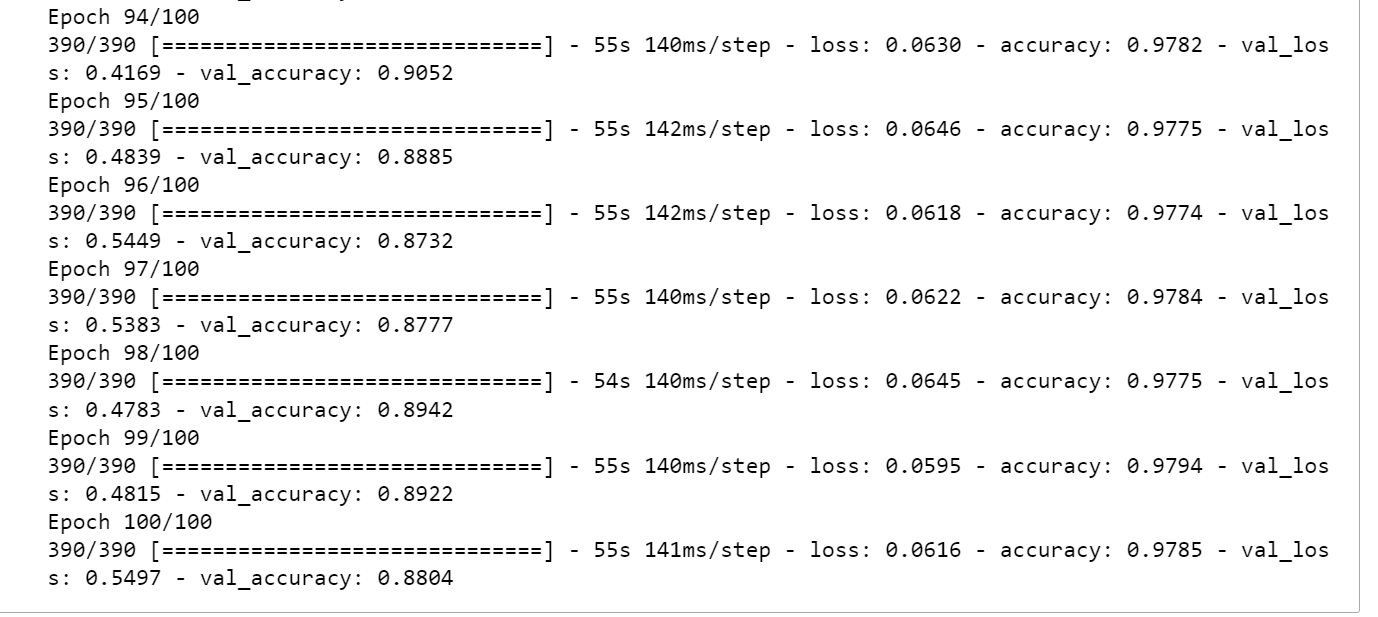
model1 = model.fit_generator(data, steps_per_epoch=step_size, epochs=100, verbose=1, validation_data=(X_test, y_test))After running the 100 epoch we got very good accuracy here-
Author GitHub
Here we saw some time accuracy is increased and the next epoch accuracy is reduced because of the local oscillation inaccuracy here accuracy is not go down at minimum points so they oscillate and take more time to go down.
Conclusion
In this session, we explored the fundamental principles of DenseNet architecture, comparing its advantages over ResNet. Unlike traditional architectures, DenseNet’s connections increase exponentially, improving information flow. Each layer in DenseNet receives input not just from the preceding layer, but from all previous layers as well, fostering enhanced learning. We delved into implementing DenseNet on the CIFAR-10 dataset, comprising 10 image classes, achieving notable accuracy. By adjusting dropout rates and layer values, we refined the model, optimizing its performance. This foundational understanding equips us to harness DenseNet’s efficacy in various applications, leveraging its unique connectivity for superior learning outcomes.


[…] post Introduction to DenseNets (Dense CNN) appeared first on Analytics […]
what is compression used for?