This article was published as a part of the Data Science Blogathon.
Table of Contents
1. Introduction to the curse of dimensionality.
2. What is PCA and why do we need it?
3. Steps in PCA and mathematical proof.
The Curse of Dimensionality
In Numpy, the number of independent features or variables in a dataset is known as a dimension.
In Mathematics, Dimension is defined as the minimum number of coordinates needed to specify a vector in space.
When we have a larger dataset in terms of features, there will be an exponential increase in computation effort needed for processing or analysis, In theory, an increase in dimension can add an extreme amount of information to data, but practically it increases noise and redundancy in the data. Distance-based machine learning algorithms won’t work well with higher dimensional data,
The formula for calculating a distance between two vectors in one dimension,Image source
The formula for calculating a distance between two vectors in two dimensions
The formula for calculating a distance between two vectors in N dimensions
We can notice that when the dimension increases we need a lot of computation to find a distance between two vectors(records), and what if we have millions of records it needs a lot of CPU cores to complete the task. In that case, a higher dimension is considered as a “curse” .e.g. KNN(k-Nearest-Neighbor) is a distance-based machine learning algorithm.
Techniques in Dimensionality Reduction
1. Feature Selection Methods.
2. Manifold Learning (e.g. t-sne, MDS, etc..)
3. Matrix Factorization (e.g PCA, Kernal PCA, etc..)
What is Principal Component Analysis? Why do we need it?
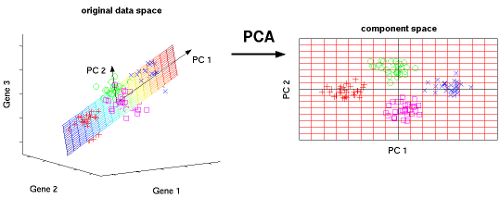
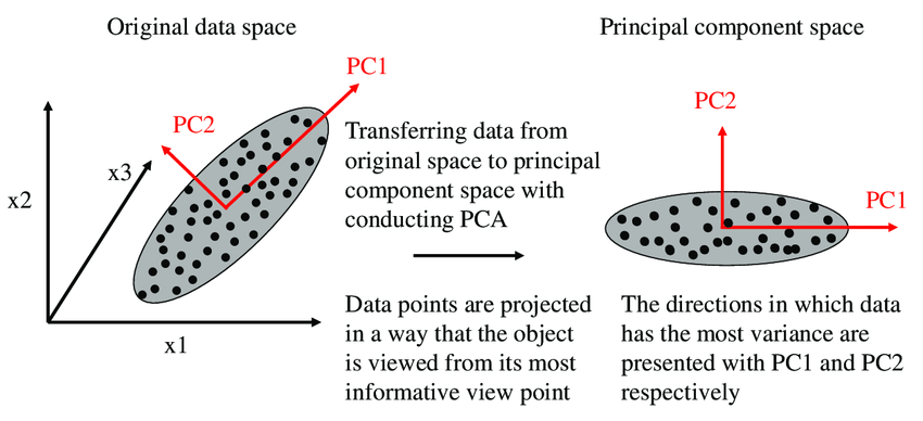
Principal Component Analysis (PCA) is a widely used dimensionality reduction technique and it comes under an unsupervised machine learning algorithm because we don’t need to provide a label for dimension reduction. We can use PCA for dimensionality reduction or we can use PCA for analysis of higher dimension data in a lower dimension. PCA algorithm’s, task is to find new axes or basis vectors that preserve a higher variance for data in lower dimensions. In PCA, new axes are known as PC’s.
In the above image, we are trying to find a new feature space in 2D for all of the vectors(data points), which are all in 3D. PC1 and PC2 are new axes for our data points. Whenever we reduce a feature(columns) in a dataset, we will lose some useful information. PCA tries to preserve the information by considering the variance of the projection vectors. Whichever vector preserves more variance, will be selected as new axes.
We can solve the PCA in two ways,
1. Select the vector which preserves more variance in the new feature space.
2. Minimizing the Error between the actual value and the projected value in the Projection vector.
Many dimensionality reduction algorithms try to preserve more information in different ways.
What is the variance of the projection vector?
I will try to break it down, projection of one vector(x) onto another vector(y), where y is known as a projection vector.
a –> a_vector
b –> b_vector
from the above image, the formula for projection of b onto a is a*b, because the length of a is 1. This is the important formula we will see where we gonna use it.
Steps in Principal Component Analysis and Mathematical Proof
Step1: Standardization of the continuous features in the dataset.
Step2: Computing the covariance matrix.
Step3: Computing eigenvalues and eigenvectors for a covariance matrix.
Why do we need a covariance matrix and eigenvalues and eigenvectors of it?
We know PCA will try to find new PCs (axes), but how is it gonna do it. it tries a bunch of vectors(xi) and tries to project all of the data points onto that vectors(xi) and it will calculate the variance of the vectors(xi) and select the vectors(xi) which preserve a higher variance of the datapoint.
Think of this like a linear regression without gradient descent, where our model will try a bunch of lines and calculate the error between the actual and prediction values. For the best fit line, we considered the cost function in linear regression. But the PCA will select the axes based on the Eigenvalues. And the axes are nothing but an Eigenvector corresponding to that eigenvalues.
New Axes = Eigenvectors
But why eigenvectors and eigenvalues ?
Before the proof, we need to understand some math formulas involved in Principal Component Analysis.
1. We need a formula for the Variance of the projection vector.
2. Need to know about a Closed-Form of the covariance.
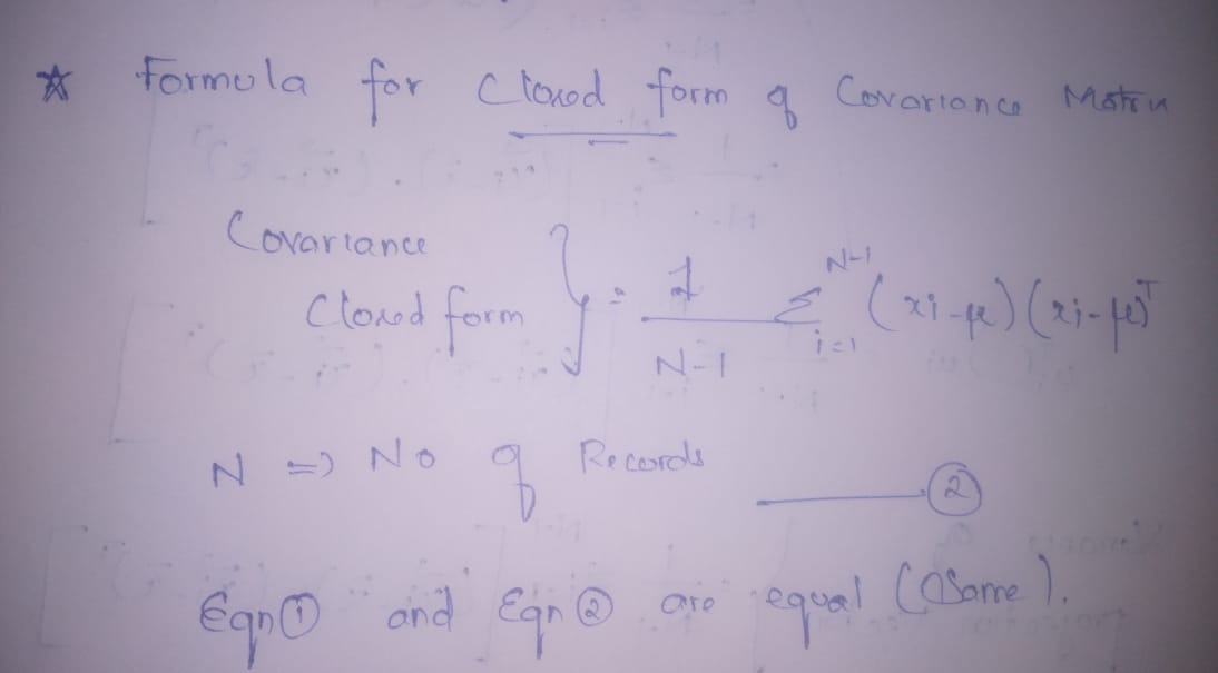
Author Image
- The formula for Closed covariance matrix. ———————-> equation 1
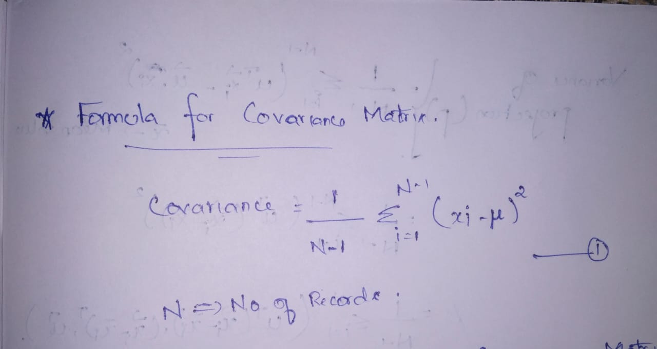
Author Image
- The formula for the Covariance matrix. —————————> equation 2
Equations 1 and 2 are the same. I am not going in-depth for the proof of the equality of covariance and closed covariance matrix.
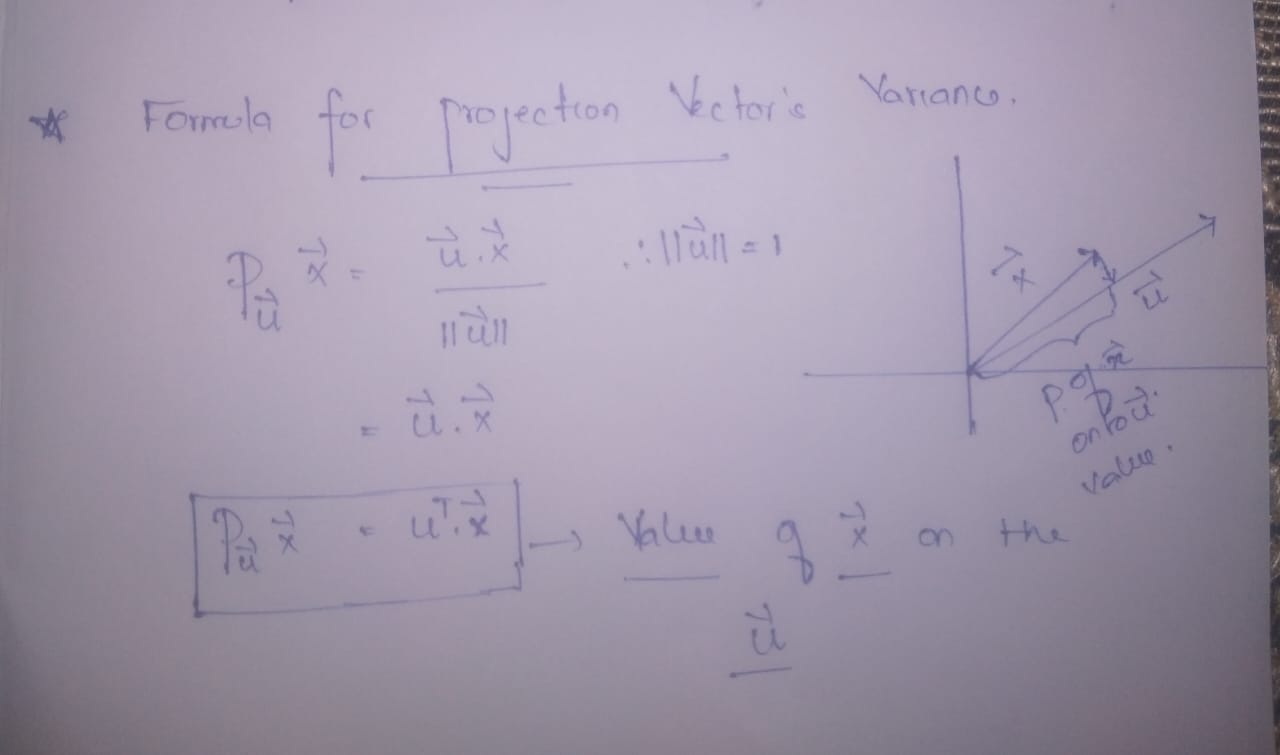
Author Image
- The formula for calculating values for data points on the new axes (PCs) —————->equation 3
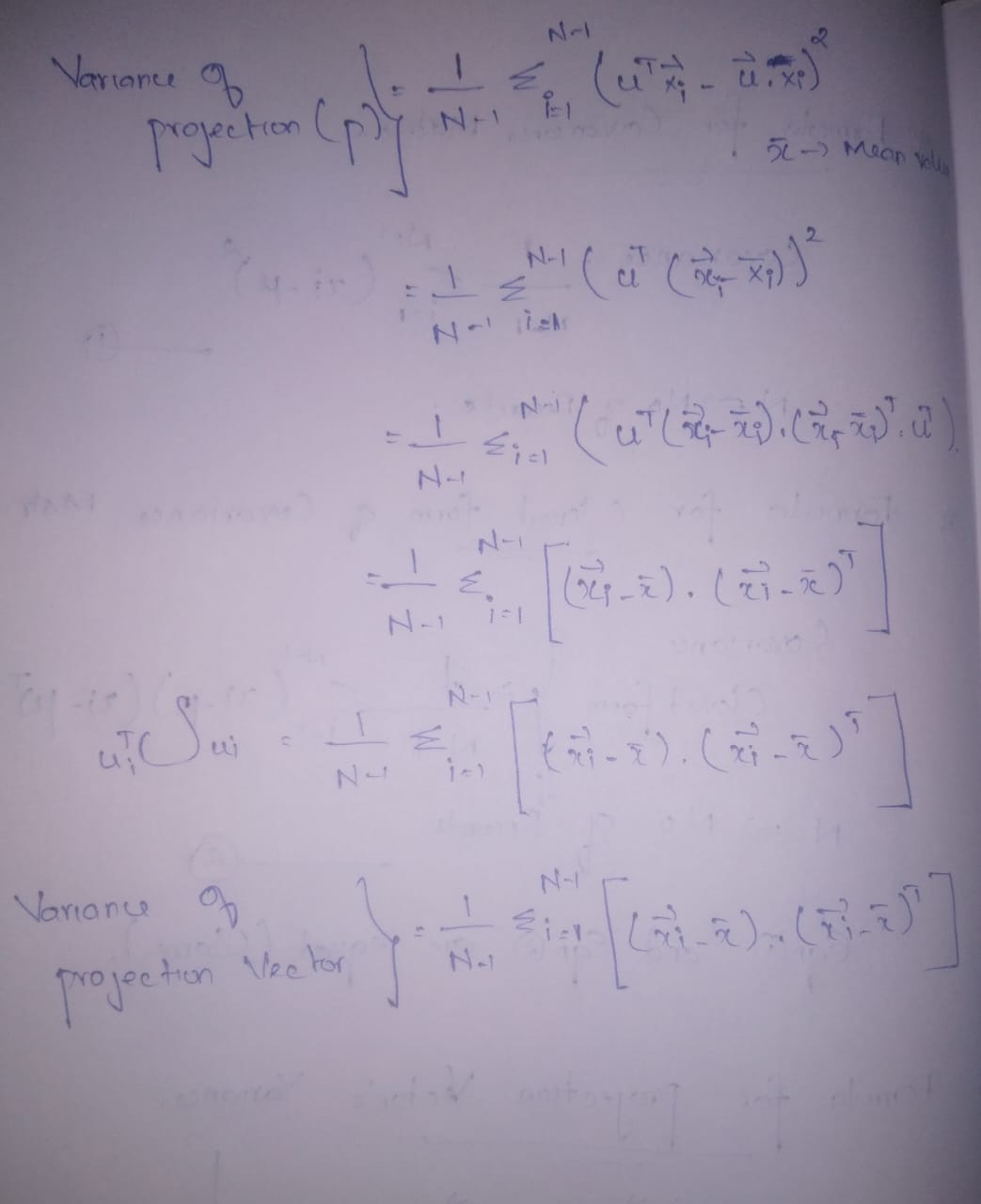
From the equation of the Variance of projection vector, we can see some magic that both closed covariance matrix and variance of projection vector are the same. So we already know that the closed covariance matrix and covariance matrix are the same. So, now variance of projection vector and covariance matrix are the same
- The covariance matrix is equal to the Variance of Projection Vector.
So this was the reason for the use of covariance matrix in PCA. And another constraint in PCA is all the axes should be orthogonal.
Why eigenvalues and eigenvectors ?
Lagrange multipliers are used in multivariable calculus for finding maxima and minima of a function that is subject to constraints.
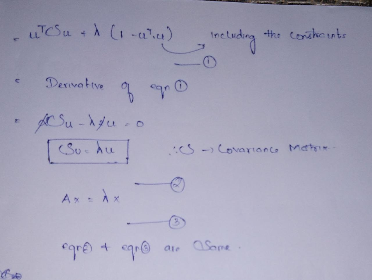
So from our linear algebra classes, we know lambda is an eigenvalue and u vector is an eigenvector, but which eigenvalue and eigenvector to select?
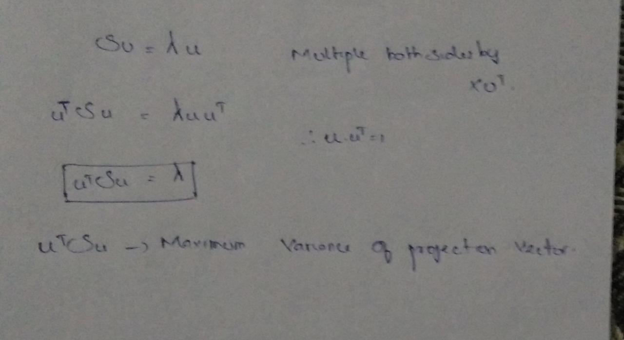
Author Image
So after some substitution, we got the maximum variance of projection vector value as Eigenvalue. So whichever vector gives the highest eigenvalues. It will be selected.
So this is the usage of covariance matrix and eigenvalues and eigenvectors.
Step 4: Sort the eigenvalues of the covariance matrix in descending order and select the n number of eigenvalues from the top. where n is the number of axes you need.
Step 5: Select the eigenvectors corresponding to the above-selected eigenvalues.
Step 6: To get the data set for the new feature space, just use the formula of Projection of data points onto new axes. U_transpose * Xi_vectors . Where U is the basis vector(axes) and Xi(data points ). Refer Equation 3.
Conclusion
- This article is mainly focused on the theoretical concepts of PCA. Which I think is most important in any dimensionality reduction techniques. So this article will give you a good basement to understand the PCA.
- So, We covered the Projection Vectors, Eigenvalues, Eigenvectors, and Why covariance matrix is used in the PCA.
- I hope, you learned how PCA works under the hood. There is some complicated math behind PCA. If you like to dig deeper into math refer to this for Lagrange Multiplier refer to the khan academy, for closed-form covariance matrix refers to this video. for projection, vectors refer to this video. to know more about PCA refer to this video on youTube. Happy Learning!
Hope you liked my article on Principal Component Analysis.
Read our latest articles on the website.




%202.jpg)