X-Ray Classification Using Pretrained-Stacked Model

This article was published as a part of the Data Science Blogathon.

Source: Link

Hey Folks!!

In the last article, we have talked about Building Search Engines using NLP concepts if you haven’t read it, refer to this link.

In this article, we are going to talk about an application of Image Classing /Classification and that is chest x-ray pneumonia prediction using the pretrained-stacked model.

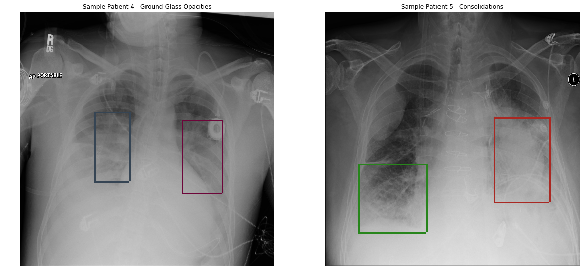
Pneumonia is caused by bacteria, fungi, and viruses. It’s a common Lung Infection. A doctor examines the X-ray and can tell if the patient is suffering from Pneumonia or not.

Streptococcus bacteria is the main cause of Pneumonia, it causes inflammation in the alveoli ( the air sacs in the lungs), and because of inflammation alveoli get filled with pus or fluid, which makes it harder to breathe.

Table of Contents

• Introduction
• Understanding the Problem
• Stacking Pretrained Model
• Implementation

Introduction

Our aim is to create a machine learning model that can categorize x-ray with pneumonia. Implementing Image Classing or Categorization can be challenging when we need to classify very fine-grained details using the pretrained-stacked model. As in our scenario, every x-ray looks very similar but in order to capture very fine details, we need to apply some different learning techniques which we are going to cover in this article.

We need to take each and every fine detail in our training to achieve our objective.

• When we used a defined CNN model we got an accuracy of 65%, It simply designates that the custom layered CNN model fails to categorize X-Ray pictures.
• To achieve higher accuracy we gonna use pre-trained stacked models.

Understanding the Dataset

We are going to use the Chest X-ray Image Dataset available on Kaggle. you can download or create a Kaggle notebook to work on it.

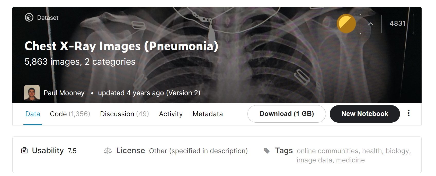
• The dataset includes training, testing, and validation data.
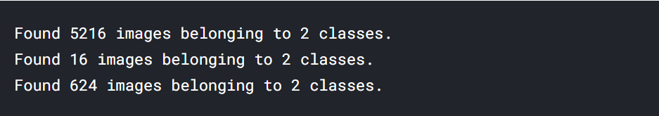
• Training data holds 5216 X-rays of which 3875 images are pneumonic and 1341 images are normal images.
• Validation data contains only 16 images including 8 normal x-rays and 8 x-rays with pneumonia.
• Testing data contains 624 images in which 390 pneumonic x-ray and 234 normal x-rays.

Implementation of X-ray Categorizer

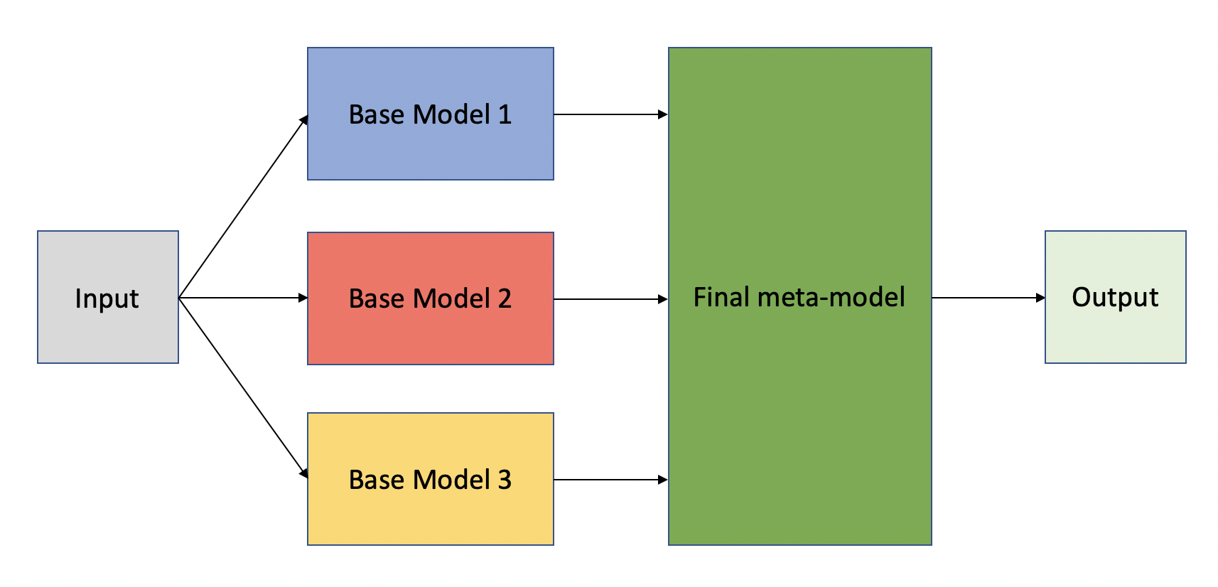
We will be using a pretrained-stacked model that is DenseNet169 and MobilenetV2 for better results.

This is done by freezing the beginning to intermediate layers of pre-trained models and then stacking them together for the output.

Step 1 Importing Libraries

We are importing all the necessary libraries at once.

from keras.layers.merge import concatenate
from keras.layers import Input
from tensorflow.keras.optimizers import Adam
from tensorflow.keras.preprocessing.image import ImageDataGenerator
from tensorflow.keras.layers import MaxPooling2D, Flatten,Conv2D, Dense,BatchNormalization,GlobalAveragePooling2D,Dropoutfrom tensorflow.keras.applications.densenet import DenseNet169
from tensorflow.keras.applications.mobilenet_v2 import MobileNetV2

Step 2 Loading the Data

The dataset contains hierarchical folders for the training images and validation. we have saved the path as variables.

• train_n(training data for normal Xray)
• train_p(training data for pneumonia Xray)
• validation_data_dir ( validation data)
• test_data_dir( for testing )

main_dir = "../input/chest-xray-pneumonia/chest_xray/"
train_data_dir = main_dir + "train/"
validation_data_dir = main_dir + "val/"
test_data_dir = main_dir + "test/"
train_n = train_data_dir+'NORMAL/'
train_p = train_data_dir+'PNEUMONIA/'

Step 3 Creating Data Generator

Since the dataset is big and to avoid memory insufficiency we need to train the model into batches, to achieve this purpose we will use a data generator.

Apart from this, we need to apply data augmentation to avoid overfitting problems.

In the data augmentation, by applying some small transformations we achieve more generalized results. this also leads to generating more training data by applying transformations on it.

The data Image data generator handles all the image processing tasks.

Note– We apply image augmentation only on the training images, not on the testing and validation images.

train_datagen = ImageDataGenerator(
    rescale=1. / 255,
    horizontal_flip=True)

test_datagen = ImageDataGenerator(rescale=1. / 255)
val_datagen = ImageDataGenerator(rescale=1. / 255)

The following image transformation can be applied ie-

• zoom_rangeFloat Value: Ranges [lower, upper]
• shear_rangeFloat Value. Shear Intensity
• rescale It is used to normalize the image

Step 4 Loading the data into DataGenerator 

The methodflow_from_directory loads the data recursively by going to the directory by directory if our main directory is in a hierarchical fashion.

img_width , img_height = [224,224]
batch_size = 16

train_generator = train_datagen.flow_from_directory(
    train_data_dir,
    target_size=(img_width, img_height),
    batch_size=batch_size,
    class_mode='binary',
    shuffle = True)

validation_generator = val_datagen.flow_from_directory(
validation_data_dir,
target_size=(img_height, img_width),
batch_size=batch_size,
class_mode=’binary’)

test_generator = test_datagen.flow_from_directory(
test_data_dir,
target_size=(img_height, img_width),
batch_size=batch_size,
class_mode=’binary’)

• class_mode = ‘binary’ since it’s a binary Categorization.
• target_size = (img_height, img_width) of the size of the target, the image is to be granted by the image data generator.
• batch_size = 16 16 images will be grouped in a batch and the model will be trained by taking the batch of images. Using batches we solve the problem of memory insufficiency.

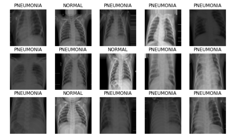
Plotting the Images Generated by Image Data Generator

image_batch, label_batch = next(iter(train_generator))

def show_batch(image_batch, label_batch):
plt.figure(figsize=(10, 10))
for n in range(15):
ax = plt.subplot(5, 5, n + 1)
plt.imshow(image_batch[n])
if label_batch[n]:
plt.title(“PNEUMONIA”)
else:
plt.title(“NORMAL”)
plt.axis(“off”)

show_batch(image_batch, label_batch)

Step 5 Model Building

We will use pre-trained DenseNet169 and MobilenetV2 and will stack the last pre-trained layers using merge class.

Freezing the top to intermediate layers means we are keeping the pre-trained weights and we are not training it from scratch.

input_shape = (224,224,3)
input_layer = Input(shape = (224, 224, 3))

#first model
mobilenet_base = MobileNetV2(weights = ‘imagenet’,input_shape = input_shape,include_top = False)

densenet_base = DenseNet169(weights = 'imagenet', input_shape = input_shape,include_top = False)

for layer in mobilenet_base.layers:
    layer.trainable =  False
for layer in densenet_base.layers:
    layer.trainable = False
    
model_mobilenet = mobilenet_base(input_layer)
model_mobilenet = GlobalAveragePooling2D()(model_mobilenet)
output_mobilenet = Flatten()(model_mobilenet)

model_densenet = densenet_base(input_layer)
model_densenet = GlobalAveragePooling2D()(model_densenet)
output_densenet = Flatten()(model_densenet)

merged = tf.keras.layers.Concatenate()([output_mobilenet, output_densenet])

x = BatchNormalization()(merged)
x = Dense(256,activation = ‘relu’)(x)
x = Dropout(0.5)(x)
x = BatchNormalization()(x)
x = Dense(128,activation = ‘relu’)(x)
x = Dropout(0.5)(x)
x = Dense(1, activation = ‘sigmoid’)(x)
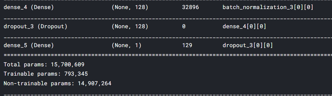
stacked_model = tf.keras.models.Model(inputs = input_layer, outputs = x)

• Freezing all the top to intermediate layers to keep the pre-trained weights and only train the model for the output after stacking.

Most of the pre-trained CNN models are trained on the imagenet dataset.

• tf.keras.layers.Concatenate() It concatenates the outputs for stacking.
• stacked_model it is the final model ready for the predictions.

Model Compilation

So far we have designed our model, its time to assign some learning parameters and compile the model.

• LR = 0.0001
• optimizer = adam

We are trying adam optimizer and LR = 0.0001, the small rate of learning is the better starting for the pre-trained model.

optm = Adam(lr=0.0001)
stacked_model.compile(loss='binary_crossentropy', optimizer=optm, 
                  metrics=['accuracy'])

Step 6 Defining Callbacks

Callbacks are a tool for efficient training, but it’s not mandatory to use, and it gives us control over the training.

from keras.callbacks import EarlyStopping,ReduceLROnPlateau
EarlyStopping = EarlyStopping(monitor='val_accuracy',
                              min_delta=.01,
                              patience=6,
                              verbose=1,
                              mode='auto',
                              baseline=None,
                              restore_best_weights=True)

EarlyStopping: It stops the training if the model doesn’t get better results after some epochs.

rlr = ReduceLROnPlateau( monitor="val_accuracy",
                            factor=0.01,
                            patience=6,
                            verbose=0,
                            mode="max",
                            min_delta=0.01)

ReduceLROnPlateau It reduces the rate of learning (LR) if the model doesn’t get better.

model_save = ModelCheckpoint('./stacked_model.h5',
                             save_best_only = True,
                             save_weights_only = False,
                             monitor = 'val_loss', 
                             mode = 'min', verbose = 1)

ModelCheckpoint : it saves the model at several epochs.

Step 7 Training

Now we are ready with the model and data, it’s time to start the training

nb_train_samples = 5216 # number of training-samples
nb_validation_samples = 16 # number of validation-samples
nb_test_samples = 624 # number of training-samples
epochs = 20  
batch_size  = 16

Training

stacked_history = stacked_model.fit(train_generator,
                              steps_per_epoch = nb_train_samples // batch_size,
                              epochs = 20,
                              validation_data = test_generator,
                           
                              callbacks=[EarlyStopping, model_save,rlr])

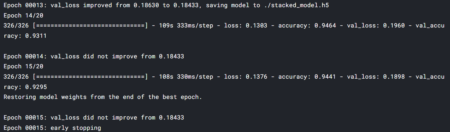
• maximum val_accuracy The maximum accuracy we have got is 93% and loss is .18 the minimum loss. The model and training can be further improved by using fine-tuning and stacking a few more dense models.

Step 8 Testing of the Model

Testing the model performance by creating a predict function inputs an image and model name and tells whether it’s a normal x-ray or pneumonic X-ray.

def process_image(image):
    image = image/255
    image = cv2.resize(image, (224,224))
    return image

The function preprocess_image() takes the image array and normalizes it by dividing it by 255 and resizing it to (224,224).

def predict(image_path, model):
    im = cv2.imread(image_path)
    test_image = np.asarray(im)
    processed_test_image = process_image(test_image)
    processed_test_image = np.expand_dims(processed_test_image, axis = 0)
    
    ps = model.predict(processed_test_image)
    return ps

The functionpredict() inputs the image path image_path and model and returns prediction.

from sklearn.metrics import classification_report,confusion_matrix

from PIL import Image

def testing(model, test_df):
base_pred =[] for image in test_df.img_path:
base_pred.append(predict(image , model)[0][0])

final_base_pred = np.where(np.array(base_pred)>0.5,1,0)
actual_label = test_df[‘label’] # print(final_base_pred)

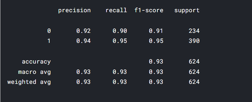
print(classification_report(actual_label, final_base_pred))
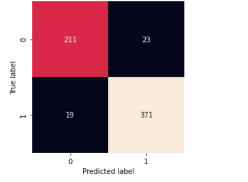
matrix=confusion_matrix(actual_label, final_base_pred)
sb.heatmap(matrix,square=True, annot=True, fmt=’d’, cbar=False,
xticklabels=[‘0’, ‘1’],
yticklabels=[‘0’, ‘1’])
plt.xlabel(‘Predicted label’)
plt.ylabel(‘True label’)

The functiontesting() is made to return the confusion matrix and training report for a better understanding of our model performance.

testing(stacked_model,test_df)

Confusion-Matrix

Conclusion

In this article, we discussed implementing the Pretrained-stacked model for our X-ray image segregation. We discussed the working of the image data generator, and using functional API we build our model and using callbacks we have trained it.

Key Points

• The stacked model we trained has the lowest loss in 20 epochs and the highest validation accuracy
• You can try (CLAHE and normalization) for better accuracy.
• Stacking a number of models with more dense architecture can promise a better result.

Hope you liked my article on the pretrained-stacked model. Feel free to hit me on Linkedin if you have something to ask about.

The media shown in this article is not owned by Analytics Vidhya and are used at the Author’s discretion. 

Abhishek Jaiswal

A data enthusiast exploring the leading technologies related to the data