Master Image Augmentation with 3 Widely Used Python Libraries

In my previous article, we explored image augmentation using AugLy, a recently introduced library from Facebook. Now, let’s delve into three popular image augmentation libraries in Python.

Grayscale, GPU, GaussianBlur, Kaggle, DataGen, Batch_Size, Algorithm, Sequential, Resizing, API:

An image classifier’s performance improves with a larger and more diverse dataset. However, gathering diverse data can be time-consuming and expensive. Image data augmentation solves this problem by generating various images for training. Techniques include geometric transformations (flipping, cropping, rotating, zooming), color transformations (brightness adjustment, saturation), and more.

We can augment the image data using various techniques. It can include:

• Augmenting image data using Geometric transformations such as flipping, cropping, rotating, zooming, etc.
• Augmenting image data by using Color transformations such as by adjusting brightness, darkness, sharpness, saturation, etc.
• Augmenting image data by random erasing, mixing images, etc.

This article was published as a part of the Data Science Blogathon.

Learning Objectives

• Understand the importance of image augmentation in machine learning tasks.
• Learn about different Python libraries for image augmentation: Imgaug, Albumentations, and SOLT.
• Gain familiarity with various image augmentation techniques and how to implement them using different libraries.
• Learn to define augmentation pipelines for efficient data augmentation.
• Understand the role of augmentation in improving model robustness and generalization capabilities.

Imgaug Tutorial

Imgaug is an open-source python package that allows you to augment images in machine learning experiments. It works with a variety of augmentation techniques. It has a simple yet powerful interface and can augment images optimizer, landmarks, bounding boxes, heatmaps, and segmentation maps.

Imgaug is a powerful library for image augmentation in machine learning experiments. It supports a variety of techniques such as flipping, rotation range, and cropping. It also allows more complex methods like adding Gaussian noise or blurring the images.

Let’s start by installing this library first using pip from PyPI.

pip install imgaug

Next, we will install the python package named ‘IPyPlot’ in the command prompt using the pip command:

pip install ipyplot

IPyPlot is a Python tool that allows for the fast and efficient display of images within Python Notebook cells. This package combines IPython with HTML to provide a quicker, richer, and more interactive way to show images. This package’s ‘plot_images’ command will be used to plot all of the images in a grid-like structure.

Also, we will import all the necessary packages needed to augment the data.

import imageio
import imgaug as ia
import imgaug.augmenters as iaa

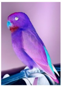
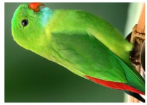
The image path for augmentation is defined here. We’ll use a bird image as an example.

input_img = imageio.imread('../input/image-bird/bird.jpg')

Image Flipping

We can flip the image horizontally and vertically using the commands shown below. ‘Fliplr’ keyword in the following code flips the image horizontally. Similarly, the keyword ‘Flipud’ flips the image vertically.

Image flipping is a simple yet effective technique used in data augmentation. It helps the model generalize better by providing it with ‘new’ images that are flipped versions of the original images in the dataset.

#Horizontal Flip
hflip= iaa.Fliplr(p=1.0)
input_hf= hflip.augment_image(input_img)

#Vertical Flip
vflip= iaa.Flipud(p=1.0) 
input_vf= vflip.augment_image(input_img)
images_list=[input_img, input_hf, input_vf]
labels = ['Original', 'Horizontally flipped', 'Vertically flipped']
ipyplot.plot_images(images_list,labels=labels,img_width=180)

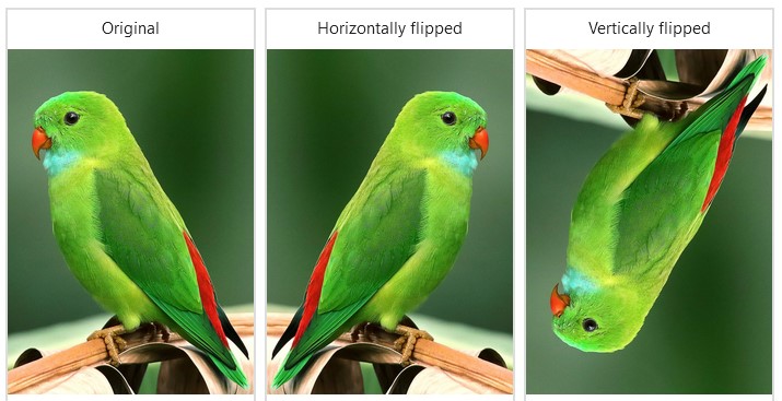
The probability of each image getting flipped is represented by p. The probability is set to 0.0 by default. To flip the input image horizontally, use Fliplr(1.0) rather than just Fliplr (). Similarly, when flipping the image vertically, use Flipud(1.0) rather than just Flipud().

Image Rotation

By defining the rotation in degrees, we can rotate the image.

Image rotation is another common technique in data augmentation. By rotating the images at various angles, we can increase the diversity of our training data and help our model become more robust.

rot1 = iaa.Affine(rotate=(-50,20))
input_rot1 = rot1.augment_image(input_img)
images_list=[input_img, input_rot1]
labels = ['Original', 'Rotated Image']
ipyplot.plot_images(images_list,labels=labels,img_width=180)

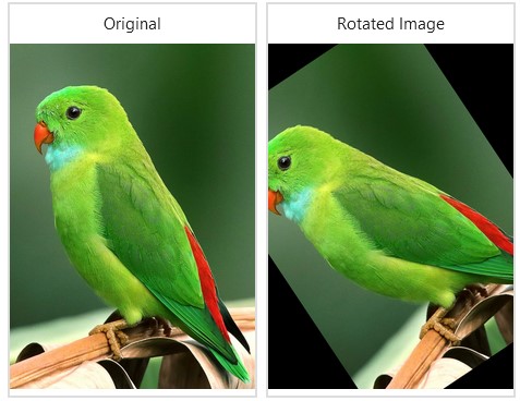
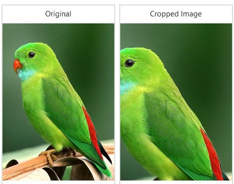
Image Cropping

Image cropping is used to focus on specific parts of an image. This is particularly useful in tasks like object detection where we want our model to recognize objects regardless of their position in the image. Cropping images includes removing columns or rows of pixels from the image’s sides. This augmenter enables the extraction of smaller-sized subimages from full-sized input images. The number of pixels to be removed can be specified in absolute numbers or as a fraction of the image size.

In this case, we crop each side of the image with a random fraction taken uniformly from the continuous interval [0.0, 0.3] and sampled once per image and side. Here, we are taking a sampled fraction of 0.3 for the top side, which will crop the image by 0.3*H, where H is the height of the input image.

crop1 = iaa.Crop(percent=(0, 0.3)) 
input_crop1 = crop1.augment_image(input_img)
images_list=[input_img, input_crop1]
labels = ['Original', 'Cropped Image']
ipyplot.plot_images(images_list,labels=labels,img_width=180)

Adding Noise to Images

Adding noise to images is a technique used to make the model more robust. It involves adding random variations to the pixel values of the images.

This augmenter adds gaussian noise to the input image. The scale value is the standard deviation of the normal distribution that generates the noise.

noise=iaa.AdditiveGaussianNoise(10,40)
input_noise=noise.augment_image(input_img)
images_list=[input_img, input_noise]
labels = ['Original', 'Gaussian Noise Image']
ipyplot.plot_images(images_list,labels=labels,img_width=180)

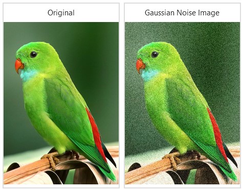
Image Shearing

Image shearing involves shifting one part of an image to a direction while keeping the other parts fixed. It’s a useful technique for training neural networks as it provides a different perspective of the data.

This augmenter shears the image by random amounts ranging from -40 to 40 degrees.

shear = iaa.Affine(shear=(-40,40))
input_shear=shear.augment_image(input_img)
images_list=[input_img, input_shear]
labels = ['Original', 'Image Shearing']
ipyplot.plot_images(images_list,labels=labels,img_width=180)

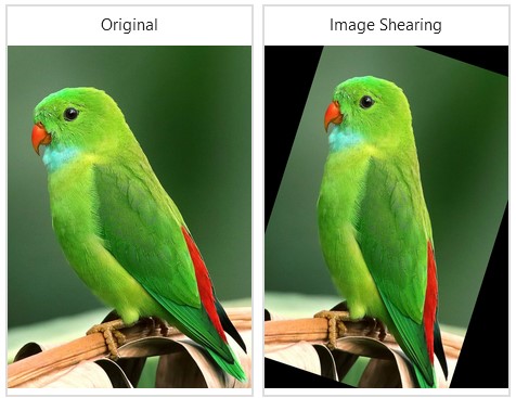
Image Contrast

Adjusting the image contrast can highlight or obscure certain features in the image. This can be beneficial in tasks like object detection or image recognition.

This augmenter adjusts the image contrast by scaling pixel values.

contrast=iaa.GammaContrast((0.5, 2.0))
contrast_sig = iaa.SigmoidContrast(gain=(5, 10), cutoff=(0.4, 0.6))
contrast_lin = iaa.LinearContrast((0.6, 0.4))
input_contrast = contrast.augment_image(input_img)
sigmoid_contrast = contrast_sig.augment_image(input_img)
linear_contrast = contrast_lin.augment_image(input_img)
images_list=[input_img, input_contrast,sigmoid_contrast,linear_contrast]
labels = ['Original', 'Gamma Contrast','SigmoidContrast','LinearContrast']
ipyplot.plot_images(images_list,labels=labels,img_width=180)

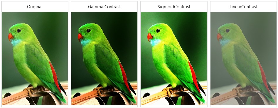
The GammaContrast function here adjusts image contrast using the formula 255*((v/255)**gamma, where v is a pixel value and gamma is evenly sampled from the range [0.5, 2.0]. SigmoidContrast adjusts image contrast using the formula 255*1/(1+exp(gain*(cutoff-v/255)) (where v is a pixel value, the gain is sampled uniformly from the interval [3, 10] (once per image), and the cutoff is sampled consistently from the interval [0.4, 0.6]. LinearContrast, on the other hand, alters image contrast using the formula 127 + alpha*(v-127)’, where v is a pixel value and alpha is sampled uniformly from the range [0.4, 0.6].

Image Transformations

Image transformations involve changing the appearance of an image using operations like translation, rotation, scaling, etc. These transformations can help improve the performance of the model by providing it with a more diverse dataset.

The ‘Elastic Transformation’ augmenter transforms images by shifting pixels around locally using displacement fields. The augmenter’s parameters are alpha and sigma. The strength of the displacement is controlled by alpha, wherein greater values indicate that pixels are shifted further. The smoothness of the displacement is controlled by sigma, in which larger values result in smoother patterns.

elastic = iaa.ElasticTransformation(alpha=60.0, sigma=4.0)
polar = iaa.WithPolarWarping(iaa.CropAndPad(percent=(-0.2, 0.7)))
jigsaw = iaa.Jigsaw(nb_rows=20, nb_cols=15, max_steps=(3, 7))
input_elastic = elastic.augment_image(input_img)
input_polar = polar.augment_image(input_img)
input_jigsaw = jigsaw.augment_image(input_img)
images_list=[input_img, input_elastic,input_polar,input_jigsaw]
labels = ['Original', 'elastic','polar','jigsaw']
ipyplot.plot_images(images_list,labels=labels,img_width=180)

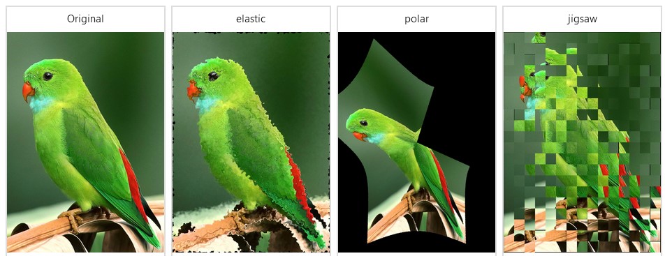
The ‘Polar Warping’ Augmenter first applies cropping and padding in polar representation, then warps the image back to cartesian representation. This augmenter can add additional pixels to the image.The augmenter will fill these additional pixels with black. In addition, the ‘Jigsaw’ augmentation moves cells inside pictures in a manner similar to jigsaw patterns.

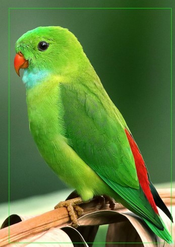
Bounding Box on Image

In object detection tasks, bounding boxes denote the location of the object in the image. Typically, they are created during the preprocessing stage before feeding the images into the model.

imgaug also provides bounding box support for images. The library can rotate all bounding boxes on an image if rotated during augmentation.

from imgaug.augmentables.bbs import BoundingBox, BoundingBoxesOnImage
bbs = BoundingBoxesOnImage([
 BoundingBox(x1=40, x2=550, y1=40, y2=780)
], shape=input_img.shape)
ia.imshow(bbs.draw_on_image(input_img))

Albumentations

Albumentations is a fast and flexible image augmentation library. Albumentations offers a wide range of augmentation techniques and is optimized for high performance, making it suitable for tasks that require heavy image processing.

Albumentations is a fast and well-known library that integrates with popular deep learning frameworks such as PyTorch and TensorFlow. It is also a part of the PyTorch ecosystem.

Albumentations can perform all typical computer vision tasks, including classification, semantic segmentation, instance segmentation, object identification, and posture estimation. This library includes over 70 different augmentations for creating new training samples from existing data. Industry, deep learning research, machine learning contests, and open-source projects commonly utilize it.

Let’s start by installing the library first using the pip command.

pip install Albumentations

We will import all the necessary packages needed for augmenting data with Albumentations:

import albumentations as A
import cv2

In addition to the Albumentations package, we use the OpenCV package, an open-source computer vision library that supports a wide range of image formats. Albumentations are dependent on OpenCV; thus, you already have it installed.

Each of these topics plays a crucial role in image processing and you can implement them using various tools like Keras, Numpy, etc. They help in preprocessing the images, augmenting the image dataset, and improving the performance of the model. Remember, the goal of these techniques is to make your model more robust and capable of generalizing from the training data to new images it has never seen before.

Image Flipping

The ‘A.HorizontalFlip’ and ‘A.VerticalFlip’ functions flip the image horizontally and vertically. Most augmentations support the parameter ‘p’, which controls the probability of the augmentation being used.

#HorizontalFlip
transform = A.HorizontalFlip(p=0.5)
augmented_image = transform(image=input_img)['image']
plt.figure(figsize=(4, 4))
plt.axis('off')
plt.imshow(augmented_image)

#VerticalFlip
transform = A.VerticalFlip(p=1)
augmented_image = transform(image=input_img)['image']
plt.figure(figsize=(4, 4))
plt.axis('off')
plt.imshow(augmented_image)

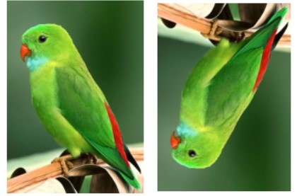
Image Scale and Rotate

This augmenter uses affine transformations at random to translate, scale, and rotate the input image.

transform = A.ShiftScaleRotate(p=0.5)
random.seed(7) 
augmented_image = transform(image=input_img)['image']
plt.figure(figsize=(4, 4))
plt.axis('off')
plt.imshow(augmented_image)

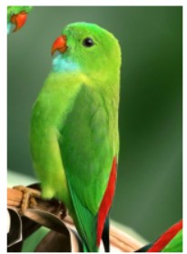
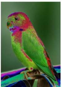
Image ChannelShuffle

This augmenter randomly rearranges the RGB channels of the input image.

from albumentations.augmentations.transforms import ChannelShuffle
transform = ChannelShuffle(p=1.0)
random.seed(7) 
augmented_image = transform(image=input_img)['image']
plt.figure(figsize=(4, 4))
plt.axis('off')
plt.imshow(augmented_image)

Image Solarize

This augmenter inverts all pixel values greater than a certain threshold in the input image.

from albumentations.augmentations.transforms import Solarize
transform = Solarize(threshold=200,  p=1.0)
augmented_image = transform(image=input_img)['image']
plt.figure(figsize=(4, 4))
plt.axis('off')
plt.imshow(augmented_image)

Invert Image

By subtracting pixel values from 255, this augmenter inverts the input image.

from albumentations.augmentations.transforms import InvertImg
transform = InvertImg(p=1.0)
augmented_image = transform(image=input_img)['image']
plt.figure(figsize=(4, 4))
plt.axis('off')
plt.imshow(augmented_image)

Augmentation pipeline using Compose

To define an augmentation pipeline, first, create a Compose instance. You must provide a list of augmentations as an argument to the Compose class. In this example, we’ll utilize a variety of augmentations such as transposition, blur, distortion, etc.

A Compose call will result in the return of a transform function that will do image augmentation.

transform = A.Compose([
    A.RandomRotate90(),
    A.Transpose(),
    A.ShiftScaleRotate(shift_limit=0.08, scale_limit=0.5, rotate_limit=5, p=.8),
    A.Blur(blur_limit=7),
    A.GridDistortion(),
])
random.seed(2) 
augmented_image = transform(image=input_img)['image']
plt.figure(figsize=(4, 4))
plt.axis('off')
plt.imshow(augmented_image)

SOLT

SOLT is a Deep Learning data augmentation library that supports images, segmentation masks, labels, and key points. SOLT is also fast and has OpenCV in its backend. Complete auto-generated documentation and examples can be found here: https://mipt-oulu.github.io/solt/.

We will start with the installation of SOLT by using the pip command –

pip install solt

Then we will import all the necessary packages of SOLT required for augmenting the image data.

import solt
import solt.transforms as slt
h, w, c = input_img.shape
img = input_img[:w]

Here we will create a Stream instance for an augmentation pipeline. You must provide a list of augmentations as an argument to the stream class.

stream = solt.Stream([
    slt.Rotate(angle_range=(-90, 90), p=1, padding='r'),
    slt.Flip(axis=1, p=0.5),
    slt.Flip(axis=0, p=0.5),
    slt.Shear(range_x=0.3, range_y=0.8, p=0.5, padding='r'),
    slt.Scale(range_x=(0.8, 1.3), padding='r', range_y=(0.8, 1.3), same=False, p=0.5),
    slt.Pad((w, h), 'r'),
    slt.Crop((w, w), 'r'),
    slt.Blur(k_size=7, blur_type='m'),
    solt.SelectiveStream([
        slt.CutOut(40, p=1),
        slt.CutOut(50, p=1),
        slt.CutOut(10, p=1),
        solt.Stream(),
        solt.Stream(),
    ], n=3),
], ignore_fast_mode=True)
fig = plt.figure(figsize=(17,17))
n_augs = 10
random.seed(2)
for i in range(n_augs):
    img_aug = stream({'image': img}, return_torch=False, ).data[0].squeeze()
    ax = fig.add_subplot(1,n_augs,i+1)
    if i == 0:
        ax.imshow(img)
    else:
        ax.imshow(img_aug)
    ax.set_xticks([])
    ax.set_yticks([])
plt.show()

Conclusion

Image augmentations can help in increasing the existing dataset. There are several Python libraries currently available for image augmentations. In this article, we have explored different image augmentation techniques using three Python libraries – Imgaug, Albumentations, and Solt.

I hope you enjoyed reading this article! The next time you train a machine learning or a deep learning model, do try one of these three libraries and the techniques shared in this article to generate additional image data quickly.

Key Takeaways

• Image augmentation is vital for improving machine learning model performance by enhancing dataset diversity.
• Python libraries like Imgaug, Albumentations, and SOLT offer powerful tools for image augmentation.
• Techniques include geometric transformations, color adjustments, noise addition, and more.
• You can efficiently define augmentation pipelines using libraries like Albumentations in Python.
• The goal is to make models more robust and capable of generalizing to unseen data.

Frequently Asked Questions

The media shown in this article is not owned by Analytics Vidhya and is used at the Author’s discretion.

Devashree

Devashree has an M.Eng degree in Information Technology from Germany and a Data Science background. As an Engineer, she enjoys working with numbers and uncovering hidden insights in diverse datasets from different sectors to build beautiful visualizations to try and solve interesting real-world machine learning problems.

In her spare time, she loves to cook, read & write, discover new Python-Machine Learning libraries or participate in coding competitions.