Introduction to Image Segmentation
This article was published as a part of the Data Science Blogathon.
Introduction on Image Segmentation
Suppose we have this image and the question that we are trying to solve is, what is the object present in this image. The object of importance here is the dog. Now, this looks like a simple enough problem, right?
This is an image classification problem. Now, instead of having a single object in the image, we can have multiple objects so our question would change accordingly.
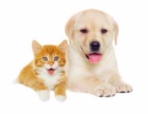
That is, what are the objects present in the image? The answer to this would be a Dog and a Cat. This is a multi-class classification task. We can identify what objects are present in the image. We can build a bounding box around the objects.
In the above image, we find a Cat & a Dog. We built a red and blue box around them respectively. But what if the question is what is the location of each pixel of the found objects?
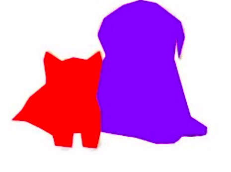
We can identify every pixel that represents the object. In simple words, instead of building a rough rectangular box around the object, we build a polygon around the object and color each pixel of that object.
What is Image Segmentation?
In simple words, “this is an image segmentation problem”. Formally speaking in image segmentation an image is divided into many segments based on the objects present and their semantic importance.
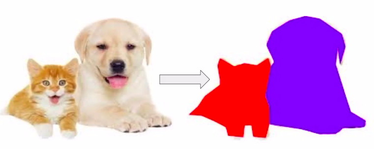
This makes it a whole lot easier to analyze the given image because instead of getting approximate locations from a rectangular box we can get the location of each pixel of found objects.
Application of Image Segmentation
Now, there are multiple applications, where image segmentation can be applied. Let us discuss a few notable applications.
Medical Imaging
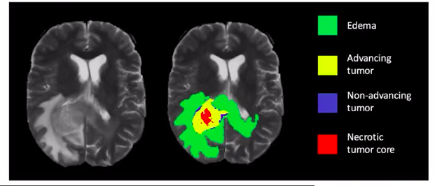
Image segmentation can be applied for medical imaging tasks e.g. “cancer cell segmentation” where it is of utmost importance that we identify each cell of the tumor or the cancerous cells.
- Cancer Cell Segmentation
- Brain Lesion Segmentation
Self Driving Cars
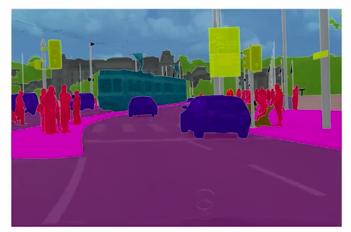
Other applications of image segmentation could be for self-driving systems, lane segmentation, or pedestrian identification. By accurately predicting the location of objects of importance like roads or a person, our self-driving system can take appropriate steps to handle the downstream tasks like applying brakes or slowing down the car.
- lane segmentation
- pedestrian identification
Satellite imaging/ Remote sensing
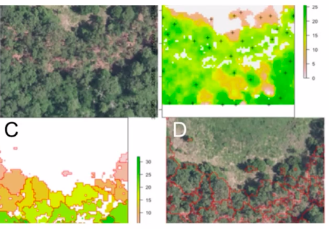
Another application could be in the “remote sensing domain”. Here we can identify a particular part of the ground e.g. forest cover in some areas. Do we have ponds or forest fires in some areas?
- Forest Area Segmentation
- Locating water bodies(lakes, rivers, oceans)
Type of Image Segmentation Problems
Now even in image segmentation, there are a few types of problems that you should be aware of.
Semantic Segmentation
Semantic segmentation describes the process of assigning every pixel of an image with a class label.
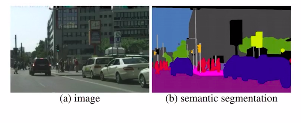
In simple words, here if you just care about a coarse representation of all the objects present in the image.
Here you can see that all the cars are represented with the color blue, the pedestrians with red, and the street slightly pink. Since all similar objects are colored the same we can not identify each object distinctly. This is one simple form of image segmentation problem. When we go one step further, we will be able to identify each object of a class. That is called instant segmentation.
Instance Segmentation
Here, we mask each object of a similar class in an image independently. It means we will only focus on the objects of importance first and then identify each object of the same class separately.
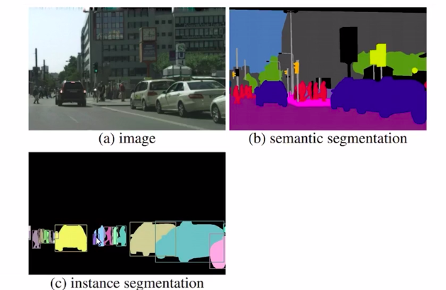
So you can see that all the objects like cars and persons are highlighted and all of these have different colors. So this is an explanation of instant segmentation. Now if you combine semantic segmentation and instant segmentation you get panoptic segmentation.
Panoptic segmentation
In Panoptic segmentation, we assign all pixels in the image with a semantic label. Which in turn can be used to identify a particular class.
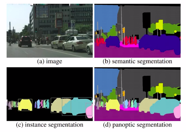
So this is a more complex problem for image segmentation. The image above clearly depicts the type of image segmentation problems discussed. Now in the next section, we’ll discuss how to solve an image segmentation problem.
How to Solve Image Segmentation?
In the previous section, we discussed what is image segmentation, which is a task of partially an image into multiple segments based on the objects present in their semantic importance.
In this section, we’ll discuss how can we solve an image segmentation problem. For this, we’ll take a problem of blood cell segmentation to understand the concepts. Let us quickly review the blood cell detection problem.
We will find the distinct WBCs in an image.
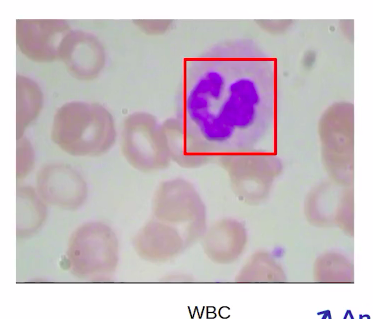
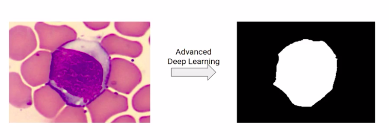
In this semantic segmentation problem, we will pinpoint the location of each cell by identifying all the pixels instead of just drawing a boundary box.
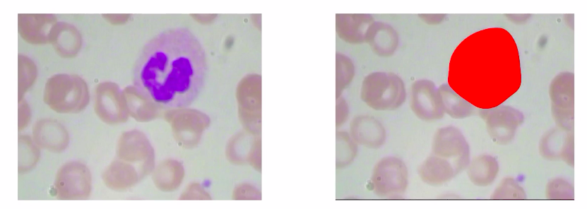
We understand that in our “use-case” using image segmentation is a better alternative to object detection because we want to identify the location of each cell rather than just drawing a bounding box around it.
So the problem, this article will be taking up is understanding the image segmentation by doing a pixel-wise classification of an image. In our data set, we have the actual image like the below image and the targets called the segmentation masks which are the colored images according to the classes.
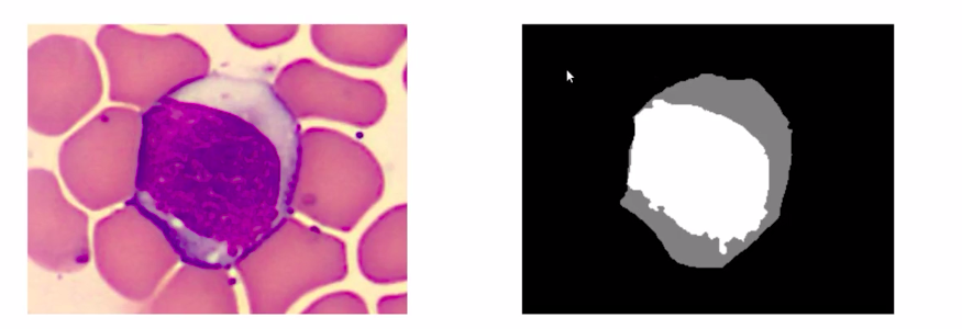
For example, the black color denotes the background class and the rest denotes the WBC.
In total, there are 100 images in our data set which is quite a small number by deep learning standards but in real life it is difficult to gather high-quality images and their annotations. As you can see here, the targets have more granular representations where the cell is colored grey and the nucleus of the cell is colored white.
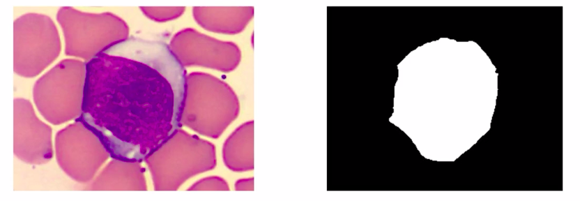
We will simplify this data to only have one class where the color white represents the class WBC and the color black represents the background. So this problem we formulated is a binary semantic segmentation problem.
The problem we choose is to identify WBCs from an image. But if we extend this idea it can potentially be applied to identifying cancerous cells. Now coming back to our question that is how to solve an image segmentation problem.

In the next few sections, we’ll discuss a few approaches to solve blood cell segmentation. There are two ways to solve this problem.
- traditional methods
- leveraging deep learning.
Approach 1 – Simple Methods (Thresholding)
In the previous section, you saw a glimpse of the problem that we formalized in order to understand image segmentation. That was segmenting WBCs in an image.
In this section specifically, we’ll discuss a few traditional but simple approaches to solve our problem at hand. Which is to have an image of a single WBC and in its background, it may have RBC’s platelets or blood plasma. We take this image and give an output image marking the part where the WBC and rest part are marked in white and black respectively.
Now, how would you approach this problem?
If we look at the image in the ‘Load Data’ section below closely, you will notice that the WBC is marked in a completely different color in comparison to the rest of the image.
So part of the image, which probably represents an RBC has a pinkish shade and, the part where WBC is present is a kind of purple. Although it is a very simple way of classifying the parts of the image differently let us use this to perform segmentation.
Now, we will use an approach like this, where we take an image convert it into a greyscale format, and then threshold it in order to perform the segmentation. Let’s move into the code walkthrough to understand this in a better way.
In segmentation, we’ll use IOU in order to compare the predictions with the actual target of the image. Also, these are the steps that we will be following in order to solve our image segmentation problem using thresholding.
Data Loading and Preprocessing
-
- Loading the Data
- Data Exploration
- Data Preprocessing
Image Segmentation through Thresholding
- Convert image to grayscale
- Apply the right threshold
- Calculate Iou Score
So let’s now move to the implementation part.
Load the Data
Let us start with loading the data from the drive. So we have to first mount the drive. Now we have two zip folders here. So first of all, we have the images for the blood cell segmentation and along with that we have targets or masks for the blood cell segmentation and these are stored in these two zip folders. So we are going to unzip these two folders so now this is going to create two new folders here.
# Upload data from drive
from google.colab import drive
drive.mount('/content/drive')
# get images
!unzip /content/drive/My Drive/images_BloodCellSegmentation.zip
# get targets
!unzip /content/drive/My Drive/targets_BloodCellSegmentation.zip
As you can see we have our images and our targets and each of these will have 100 images.
Also, BMP is a file format that is used to store the images similar to png or jpg, etc.
Data Exploration
Let’s now go ahead and explore the data. For this, we are going to first import libraries that we will use. So we have “numpy” and “matplotlib” here.
%matplotlib inline
import numpy as np
import matplotlib.pyplot as plt
from PIL import Image
from skimage.color import rgb2gray
Now, we are going to read a sample image from the dataset using the .open function and store it in a variable “img”.
# read sample image
img = Image.open('/content/images_BloodCellSegmentation/002.bmp')
Now we are going to plot this image using the “imshow” function from “matplotlib“. So here is our sample image.
# plot image
plt.imshow(img)
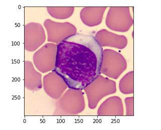
And if we print the type for this image we’ll see that this is a BMP image.
# print type
type(img)
Now we are going to convert this image into a NumPy array using the dot array function and print the shape for this image.
We can see that the shape of the image is (300, 300, 3).
# convert to numpy array
img = np.array(img)
# print shape of image
img.shape
Now we can do similar steps for our target image, which is the ground truth segmentation masks. So here we are first loading a sample from the target image and then we are going to view this target image.
# read sample target
gt_mask = Image.open('/content/targets_BloodCellSegmentation/002.png')
# plot target
plt.imshow(gt_mask, cmap='gray')
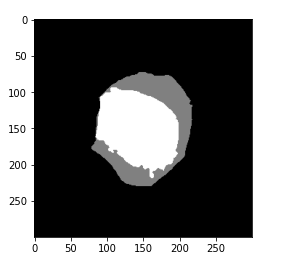
So here we can see that we have a mask that represents our WBC and the background. Now we are going to convert this into a NumPy array and print the shape for this mask.
# convert to numpy array
gt_mask = np.array(gt_mask)
# print target shape
gt_mask.shape
so we can see that the shape of the mask is (300,300) because it is already in the grayscale format. Also, note that the shape of the mask and image is the same.
Now let us move to the next section which is data preprocessing. So if you see here our ground truth mask has more granular segmentation.
Data Preprocessing
Instead of this, we would need to simplify the data. So we need only two colors to represent the mask. Black for the background and White for the WBC. But here in the mask, we have our nucleus and the WBC cell are dissociated. Let us first print out what are the unique values which are present in our mask and we are going to use the unique function here.
# get unique values
np.unique(gt_mask)
So we can see that there are three unique values zero which represents the background or the color black and we have 128 which represents the color grey and 255 which represents the color white or the nucleus of the WBC. So we are going to combine the grey and white color using the code.
# simplify unique values
gt_mask = ((gt_mask == 128) | (gt_mask == 255)).astype(int)
# get unique values again
np.unique(gt_mask)
So here we will convert both of these grey and white with white.
# plot cleaned target
plt.imshow(gt_mask, cmap='gray')
Now if you check the number of unique values. So now we have only two unique values representing the black color or the background and the WBC. Let’s print the mask in order to check if our preprocessing is successful.
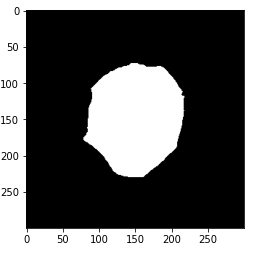
So we can see that we have only two colors in this mask now. Let us perform the thresholding we have already discussed.
Image Segmentation through Thresholding

So we will first convert the image into a grayscale format and then
threshold it. To convert the image into the grayscale format we are
going to use the RGB to grey function which is available in the “scikit” image library.
Convert Image to Grayscale
Using this function we have to input an RGB image and it
will convert this image into a grayscale format.
# convert color image to grayscale
gray = rgb2gray(img)
Let us quickly plot the image and see if this works. We can see that our original sample image which was of this format is now converted into a grayscale format.
# plot image
plt.imshow(gray, cmap='gray')
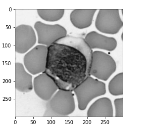
Now we are going to use the thresholding here.
Apply the Right Threshold
So first, let us find out what is the mean value for the above image.
# get mean
gray.mean()
So for the grayscale image, we can see that the mean value is 0.624.
Now our next step is to apply a threshold value. So for this, we can take the mean value of the grayscale image. To apply the threshold will first make a copy of the grayscale image to a new variable which is called mask and apply the threshold.
# make another numpy array of same values
mask = gray.copy()
# apply threshold
mask = (mask < gray.mean()).astype(int)
We have been plotting the predicted mask and we have made the prediction using the thresholding.
# plot prediction
plt.imshow(mask, cmap='gray')
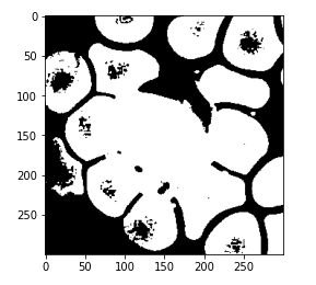
And here is the predicted mask so this is not quite the result that we expected and this may be because we didn’t define our threshold correctly.
Let us try to change the threshold value. So we will keep 0.9 this time and apply the same process. So on the image, we are going to apply a threshold of 0.9.
# Try for a different threshold
## make another numpy array of same values
mask = gray.copy()
## apply threshold
mask = (mask < 0.9).astype(int)
## plot prediction
plt.imshow(mask, cmap='gray')
We see that the performance is not getting better since more regions are now predicted incorrectly.
Let us now go ahead and change this threshold value. So I am replacing 0.9 with 0.4 and let us see what are the results.
# Try for a different threshold
## make another numpy array of same values
mask = gray.copy()
## apply threshold
mask = (mask < 0.4).astype(int)
## plot prediction
plt.imshow(mask, cmap='gray')
So now, after a trial and error, we can see that 0.4 comes out to be an appropriate threshold and we can see that this is now performing better. As we are able to now separate our WBC from the rest of the image.
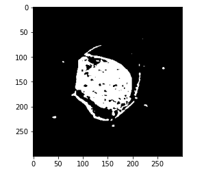
Now to evaluate how our model is performing we will calculate an IOU score for this mask.
Calculate IOU Score
For this, we first make a new “numpy” array for the predictions and the mask which is nothing but the flattened arrays of the original ones.
# make new numpy array of same values
pred = mask.ravel().copy()
target = gt_mask.ravel().copy()
We will then calculate the indices where the class of WBC that is 1 is presented for both the target and the predictions.
# get class indices for WBC
pred_inds = pred == 1
target_inds = target == 1
And then we compare these index values in order to get the intersection so let us quickly do that.
intersection = pred_inds[target_inds].sum()
print(intersection)
Now this intersection comes out to be and then the union is 16392.
union = pred_inds.sum() + target_inds.sum() - intersection
print(union)
So finally, we can calculate the intersection by the union to get an IOU score which is around 0.6. So this is a good benchmark for solving the blood cell segmentation problem.
Now let us go through the pros and cons of this approach.
Pros:-
- Simple Approach – Easy to understand
Cons:-
- Involves hard coding threshold values
- Thresholds are not the same for separate images
- Same color for separate objects
There is a better approach using clustering that is simple and solves our problem. So we are going to discuss that in the next section.
Approach 2 – Simple Methods (Clustering)
Earlier we saw a way to solve our blood cell segmentation problem, called thresholding. It was quite easy but it is done using the manual intervention.
Let us reassess our approach to image segmentation. So we saw that color is a good feature to separate our WBC from the rest of the background.
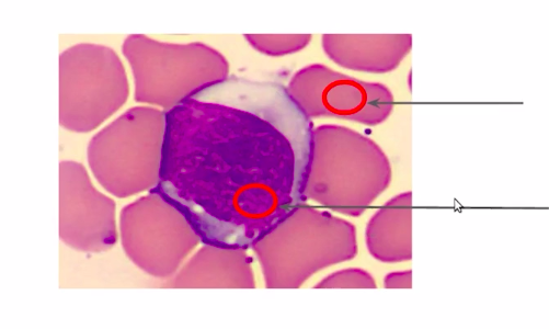
So instead of doing it manually or defining a threshold to differentiate the regions, we can group them on the basis of their color.
For example, we can take the image and find the groups of similar-looking regions and then filter out our category of interest.

This seems more intuitive than just manual thresholding. So before going to the implementation part, let us have a quick walkthrough of the steps that we will follow.
Data Loading and Preprocessing
-
- Loading the Data
- Data Extraction
- Data Cleaning
Image Segmentation through Clustering
- Apply k-means clustering on the image
- Filter the appropriate category
- Calculate Iou Score
Let us now jump into the code and understand this in a better way. So these are the steps that we are going to follow while implementing.
Load the Data
Now we are going to start by loading our data set from the drive then we are going to unzip the data sets.
# Upload data from drive
from google.colab import drive
drive.mount('/content/drive')
# get images
!unzip /content/drive/My Drive/images_BloodCellSegmentation.zip
Data Extraction
Here we have imported the libraries “numpy”, “matplotlib” etc. Also, note that here we have imported k-means clustering from sklearn. So, we used sklearn. cluster module to import k-means.
%matplotlib inline
import numpy as np
import matplotlib.pyplot as plt
from PIL import Image
from sklearn.cluster import KMeans
Now we read a sample image and have a look at the sample image to understand what the data set looks like.
img = Image.open('/content/images_BloodCellSegmentation/002.bmp')
# plot image
plt.imshow(img)
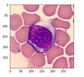
Above is the sample image. We print the type of this image and see that this is a “bmp” image file.
type(img)
output:-
PIL.BmpImagePlugin.BmpImageFile
Now we convert this image into a “numpy” array and print the shape.
img = np.array(img)
img.shape
So we can see that the shape of the input image is (300, 300,3). Now, we are going to do the same steps for our target or our mask. So, we load a sample target from the data set and look at the sample target to understand what it looks like. We can see that we have a grayscale image with three different colors.
# read sample target
gt_mask = Image.open('/content/targets_BloodCellSegmentation/002.png')
# plot target
plt.imshow(gt_mask, cmap='gray')
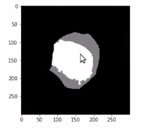
Here we are converting it into a “numpy” array and printing the shape.
# convert to numpy array
gt_mask = np.array(gt_mask)
# print target shape
gt_mask.shape
Data Preprocessing
We’ll need to preprocess this data, since we do not need this granular segmentation for our image, and we only need two things the WBC and the background.
So here we check the number of unique values in the mask and then we assign 128 and 255 in order to simplify this part. Hereafter preprocessing, we can see that we have only two unique values.
# get unique values
np.unique(gt_mask)
output:— array([ 0, 128, 255], dtype=uint8)
# simplify unique values
gt_mask = ((gt_mask == 128) | (gt_mask == 255)).astype(int)
# get unique values again
np.unique(gt_mask)
if you print the image it will look something like this.
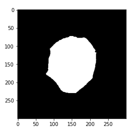
# plot cleaned target
plt.imshow(gt_mask, cmap='gray')
So this is our new target for each of these images.
Image Segmentation Through Clustering
Now let us perform clustering for image segmentation.
Apply k-means Clustering on the Image
Now, we’ll first put each pixel into clusters. and filter out our category of interest. To do this, we first initialize the k means algorithm with the number of clusters 5, and the “random_state” set to zero. Then we reshape the image to combine the height and width. We do this so that we can perform clustering on the image data.
kmeans = KMeans(n_clusters=5, random_state=0)
reshaped_image = img.reshape(img.shape[0]*img.shape[1], img.shape[2])
reshaped_image.shape
Now, the shape comes out to be (90000, 3). We will train our k-means model. Using k-means. fit.
kmeans.fit(reshaped_image)

So our k-means model goes through each of these pixel values and clusters them on the basis of their color similarity. The output that it gives is the name of the clusters for each of these pixel values. So, for the first-pixel value, the clusters are assigned with 0, then again for the second with 0, and so on.
kmeans.labels_
array([0, 0, 0, ..., 4, 4, 4], dtype=int32)
So, in this way, we will have five clusters since we have set our number of clusters to be five. Now, let us print the shape of the categories. So we can see that we have 90000 predicted values and this represents our mask.
kmeans.labels_.shape
So we can reshape this output and plot it.
# reshape labels to mask
mask = kmeans.labels_
mask = mask.reshape(img.shape[0], img.shape[1])
# print shape of mask
mask.shape
# print mask
plt.imshow(mask, cmap='gray')
Here we are reshaping our output, and then we are plotting this. So, this is the plot for our image or this is the predicted mask.
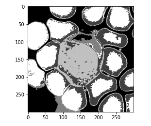
So, we can see that the model is able to separate the categories but it is giving us more classes than we expected. As you already know, we just need to separate our wbcs from the background. So instead, we are going to re-initialize our model, and this time we are going to give it clusters with 2 and then repeat the same steps.
kmeans = KMeans(n_clusters=2, random_state=0)
kmeans.fit(reshaped_image)
mask = kmeans.labels_
mask = mask.reshape(img.shape[0], img.shape[1])
plt.imshow(mask, cmap='gray')
So we have initialized the number of clusters with 2, the random_state with 0. Then we are going to train our model using the dot fit function and finally take our targets from this model and reshape it in a 300 cross 300 format and print this predicted value or the predicted mask.
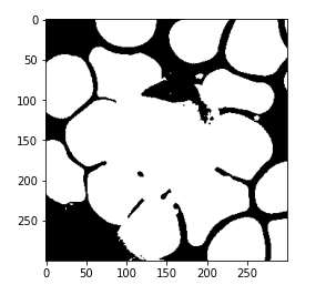
Now again, if you notice the above image, this model has successfully differentiated the RBCs and WBCs from the background. Here, we just need to separate the WBCs. So instead of assigning the number of clusters with 2, we are going to now assign the number of clusters with 3 and perform the same steps that are to train the model and reshape it.
kmeans = KMeans(n_clusters=3, random_state=0)
# train kmeans model
kmeans.fit(reshaped_image)
# reshape labels to mask
mask = kmeans.labels_
mask = mask.reshape(img.shape[0], img.shape[1])
plt.imshow(mask, cmap='gray')
Now we can see that in the below image, this model has successfully differentiated the background of the RBCs and the WBCs.
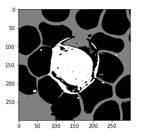
So the next step would be to filter out the appropriate category that we are interested in. And we only want the wbcs and not the RBCs or the background.
Filter the Appropriate Category
Let us quickly look at the categories manually that our model has assigned.
# get pixels with category 0
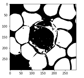
mask = (kmeans.labels_ == 0).astype(int)
mask = mask.reshape(img.shape[0], img.shape[1])
plt.imshow(mask, cmap='gray')
So here, we are only printing label 0 and we can see that 0 is assigned to all the RBCs.
Let’s see the label 1.
mask = (kmeans.labels_ == 1).astype(int)
mask = mask.reshape(img.shape[0], img.shape[1])
plt.imshow(mask, cmap='gray')
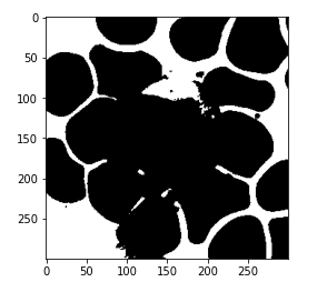
And if we print the category two this looks like our WBC class.
# get pixels with category 2
mask = (kmeans.labels_ == 2).astype(int)
mask = mask.reshape(img.shape[0], img.shape[1])
plt.imshow(mask, cmap='gray')
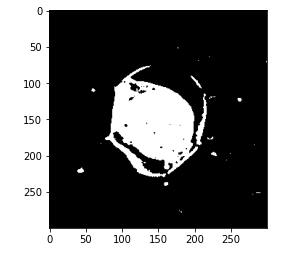
So, for this class specifically and our predicted mask should only be category 2. Now, we are going to use this mask and compare the performance of this output with the actual masks that we already have.
Calculate Iou Score
So again, we are going to use the IOU metric. This is the same code that we used in the threshold section.
# make new numpy array of same values
pred = mask.ravel().copy()
target = gt_mask.ravel().copy()
# get class indices for WBC
pred_inds = pred == 1
target_inds = target == 1
# calculate intersection
intersection = pred_inds[target_inds].sum()
# calculate union
union = pred_inds.sum() + target_inds.sum() - intersection
# get IoU score
iou = (float(intersection) / float(max(union, 1)))
iou
you can see that the IOU is 0.68, which is slightly better than earlier. So this proves that our approach is slightly better than earlier.
Let us now understand the pros and cons of this approach.
Pros:-
- Simple Approach
- Performs better than thresholding
- Can be applied to multiple images
Cons:-
- Manual filtering for labels
- Same color with different labels
- Doesn’t scale for large datasets
So, for larger data sets, this approach will not scale. So we are back to square one.
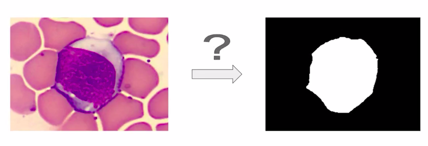
A few more traditional techniques have been applied to solve image segmentation problems which can be used here like the edge-detection or the selective search algorithm.
But for that, we would need an intelligent algorithm, that captures the semantic meaning of the pixels and classifies them accordingly to perform image segmentation. And that’s where deep learning comes into play.
In the next few articles, we’ll explore deep learning-based approaches in order to solve the blood cell segmentation problem.
Lane Segmentation for Self Driving Systems
Till now we have discussed what is image segmentation, and how to solve an image segmentation problem. In the next sections, we’ll take up a full-fledged project of lane segmentation and apply the concepts that we have learned in this article.
For example, suppose you need the tech team for a self-driving car company and the problem that you face while creating a system are understanding where to drive when to stop when to speed up, how much distance to keep between the consecutive cars, and so on.
So the problem here is to understand the scene. Let us convert this to a data science problem which will be a multi-class semantic segmentation problem.
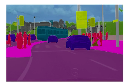
And for simplification, we are going to focus on only one problem which is where is the road?
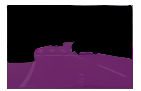
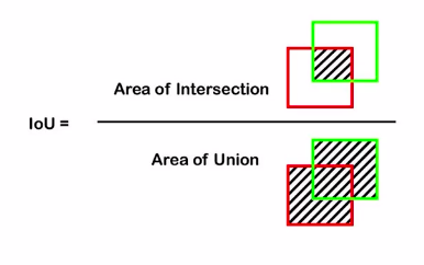
So this will become a binary semantic segmentation problem. Now we saw earlier how the evaluation metric IOU is used for evaluating the performance and here we calculate intersection and union and compare these two in order to find out how accurate the model predictions are.
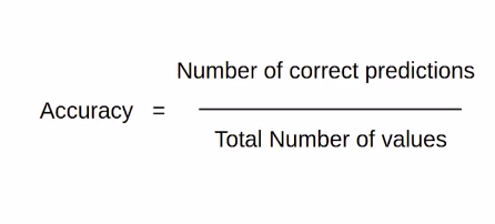
There is another popularly used metric which is called pixel accuracy. As the name suggests it describes the pixel-wise accuracy by comparing the predictions and the ground truth mask.
Now we are going to take up the lane segmentation problem. We are going to look at how can we use deep learning models like FCN, U-Net, deep lab, etc. in order to solve this lane segmentation problem.
So the loss functions that we’ll be using to train the model are binary cross-entropy and Dice Score.
We will use the dice score, which is nothing but two into the intersection upon the “total area”. So the formula is similar to IOU.
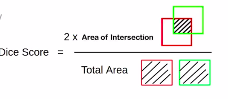
But notice that instead of the union in the denominator, “total-area” is the denominator.
Now, you might be wondering, when would someone use the Dice score? So the dice score is preferred over IOU when we care about the pixel-wise accuracy because the dice score and the IOU are positively correlated.
Now in the next section, we are going to build deep learning models and learn how to solve this task.
Solving Lane Segmentation Problems Using Fully Convolutional Network FCN
In this section, we are going to build our first model on the lane segmentation problem statement that we discussed the first model that we’ll build is the FCN model and these are the steps that we are going to follow through implementation.
Data Loading and Preprocessing
- Load the Data
- Custom dataset
- Data Exploration
Lane Segmentation using FCN
- Define model architecture
- Train the model
- Calculate IOU Score
So let’s get started.
Data Loading and Preprocessing
Load the Data
let’s start with loading the data and we’re going to mount the drive first. So we’ll first mount the drive and since the data set is in the zip format on the drive, we’ll unzip it.
# Upload data from drive
from google.colab import drive
drive.mount('/content/drive')
!unzip drive/My Drive/dataset_camVid.zip
So here we got our train images then the validation images and the validation annotations.
Once the dataset loading is done, we’ll load libraries, and these are all the libraries that we have used.
# import libraries and modules
%matplotlib inline
import os
import torch
import numpy as np
import matplotlib.pyplot as plt
from PIL import Image
from random import random
# import pytorch related modules
from torch.utils.data import Dataset, DataLoader
from torchvision.transforms import Compose, ToTensor, Resize
from torch.nn import Sequential
from torch.nn import Conv2d, ReLU, Sigmoid, BatchNorm2d, Dropout
from torchvision.models.segmentation import fcn_resnet101
from torchvision.models.segmentation.deeplabv3 import DeepLabHead
you’ll see that we have the FCN imported here. Then we set a random seed value.
# set seed
seed = 42
np.random.seed(seed)
torch.manual_seed(seed);
And defining the paths for our training validation and test sets.
x_train_dir = '/content/data/CamVid/train'
y_train_dir = '/content/data/CamVid/trainannot'
x_val_dir = '/content/data/CamVid/val'
y_val_dir = '/content/data/CamVid/valannot'
x_test_dir = '/content/data/CamVid/test'
y_test_dir = '/content/data/CamVid/testannot'
Custom Dataset
Here, we have defined the init(), get_item() and len() functions. So you can see that here we are providing a path for loading the train and validation images and masks. So, for the training, and the validation set, images, and masks, we have defined the following pre-processing steps, and then for the test set we’ll have only the images, so we have read the images, and then, our Len function.
class CamVidDataset(Dataset):
    def __init__(self, images_dir, masks_dir=None, transforms=None,
                             training_type=None):
        # get all image names
        self.image_names = os.listdir(images_dir)
        # set training type, transforms
        self.training_type = training_type
        self.transforms = transforms
        # get image and target paths
        self.images_paths = []
        self.masks_paths = []
        for image_name in self.image_names:
            self.images_paths.append(os.path.join(images_dir, image_name))
            if self.training_type=="train" or self.training_type=="val":
                self.masks_paths.append(os.path.join(masks_dir,
                                        image_name.split('.')[0] + '.png'))

    def __getitem__(self, i):

        if self.training_type=="train" or self.training_type=="val":
            # read data
            image = Image.open(self.images_paths[i])
            mask = Image.open(self.masks_paths[i])
            # preprocess mask
            mask = np.array(mask)
            mask = (mask == 3)
            mask = Image.fromarray(mask)
            # apply transforms
            image = self.transforms(image)
            mask = self.transforms(mask)

            return image, mask

        else:
            # read data
            image = Image.open(self.images_fps[i])

            # apply transforms
            image = self.transforms(image)

            return image

    def __len__(self):
        return len(self.image_names)
Data Exploration
Now, let us quickly look at a few images from the data set. So first of all we’ll set the transformations to be applied and then using our defined class we are going to pass in the image along with the transformations to be applied and take out a single image and its mask.
train_transforms = Compose([
    Resize((224, 224)),
    ToTensor()
])
dataset = CamVidDataset(x_train_dir, y_train_dir,
                         transforms=train_transforms, training_type='train')
image, gt_mask = dataset[0]
Now here we check the shape of the image and the mask.
image.shape, gt_mask.shape
So we can see that the shape of the image is (3,224, 224) and the mask is grayscale with the shape of (1,224,224).
plt.imshow(np.transpose(image, (1, 2, 0)))
Let’s plot the image and the mask.
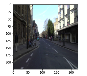
So, here is the image from the data set and you can see that the mask is segmenting the lane from the image.
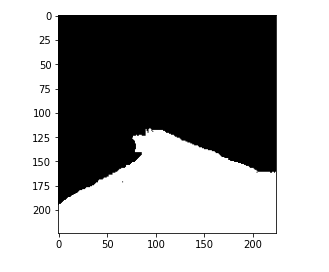
So, this is the data set that we have. I encourage you that you go ahead and check out a few more images along with the masks that you have for these training and validation sets.
Now like we did for the training set we’ll have to define the same transformations and load our validation set. . We have our transformations the class that we defined and the data loader function which will load the images in batches of 16.
train_transforms = Compose([
    Resize((224, 224)),
    ToTensor()
])

train_dataset = CamVidDataset(
    x_train_dir,
    y_train_dir,
    transforms=train_transforms,
    training_type='train'
)

train_loader = DataLoader(
    train_dataset,
    batch_size=16,
    num_workers=4
)
Then to check if the train loader is working fine, we will run this for one iteration.
for batch_x, batch_y in train_loader:
    break
Then we’ll check the batches. We can see that we have 16 images and 16 masks along with it.
batch_x.shape, batch_y.shape
The output is:-
(torch.Size([16, 3, 224, 224]), torch.Size([16, 1, 224, 224]))
Lane Segmentation Using FCN
Define Model Architecture
Let us now define the model architecture. So we are going to use the FCN architecture here and the pre-trained weights along with that and will print the model architecture.
# define model
model = fcn_resnet101(pretrained=True)
# print model
model
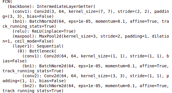
So this is the model architecture that we will use and here we have our classifier for the FCN head.
Now, we are going to use the pre-trained weights and freeze these pre-trained weights. This is called transfer learning.
# freeze model parameters
for parameters in model.parameters():
    parameters.requires_grad = False
Also based on our architecture we’ll have to update the last few layers of this model. So we’ll have to add new layers. It will be based on the number of classes that we have and here we have a single class.
model.classifier = Sequential(
    Conv2d(2048, 512, kernel_size=(3, 3), stride=(1, 1), padding=(1, 1),
                             bias=False),
    BatchNorm2d(512, eps=1e-05, momentum=0.1, affine=True,
                        track_running_stats=True),
    ReLU(),
    Dropout(p=0.1, inplace=False),
    Conv2d(512, 1, kernel_size=(1, 1), stride=(1, 1)),
    Sigmoid()
)
So we have defined the output layer and the sigmoid activation function for this layer. And let us check if the model is working fine.
# check for one iteration of loop
for batch_x, batch_y in train_loader:
    break
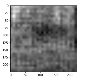
So we are going to pass a single image to the model and print the output from the model.
# check model on one image
model.eval()
output = model(batch_x[1].view(1, 3, 224, 224))['out'].detach().numpy()
# print output
plt.imshow(output.squeeze(), cmap='gray')
So, we can see that the output is the grayscale image of the shape (224, 224).
Train the Model
Now we know that the model is working fine let us train the complete model. So we are first transferring the model to GPU and defining loss function and optimizers. As we have already discussed we are going to freeze a few layers and only train the last layers for this model architecture.
# transfer model to GPU
model = model.to("cuda")
# define optimization and loss function
criterion = torch.nn.BCELoss()
optimizer = torch.optim.Adam([parameters for parameters in model.parameters()
                                 if parameters.requires_grad], lr=1e-3)
Now, after defining the optimizer and loss function will train the model. So, we are training this model for five epochs and we have initialized the loss with zero then we are taking the batches from our train loader and training the model for these batches and calculating the loss. We print the loss for each epoch.
# set model to train
model.train()
# train model
for epoch in range(5):
    # initialize variables
    epoch_loss = cnt = 0
    # loop through the data
    for batch_x, batch_y in train_loader:
        # get batch images and targets and transfer them to GPU
        batch_x = batch_x.to("cuda").float()
        batch_y = batch_y.to("cuda").float()
        # clear gradients
        optimizer.zero_grad()
        # pass images to model
        outputs = model(batch_x)
        # get loss
        loss = criterion(outputs['out'], batch_y)
        # do a backward pass
        loss.backward()
        # update gradients
        optimizer.step()
        # sum loss and get count
        epoch_loss += loss.item()
        cnt += 1
    # take average loss for all batches
    epoch_loss /= cnt

    # print loss
    print("Training loss for epoch {} is {} ".format(epoch + 1, epoch_loss))
So we have successfully trained this model.
Calculate IOU Score
Now, let us take a sample image from our training data and evaluate the model performance that is we are going to check how the model predicts for this image.
# get sample data
image = Image.open('/content/data/CamVid/train/0006R0_f00930.png')
gt_mask = Image.open('/content/data/CamVid/trainannot/0006R0_f00930.png')
So let’s first look at the original image. So, you can see that we have this image for our model.
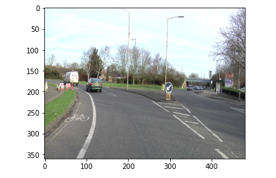
The above image will be input into our model. Let’s see what the predictions are from the model.
# preprocess mask
gt_mask = np.array(gt_mask)
gt_mask = (gt_mask == 3)
gt_mask = Image.fromarray(gt_mask)
# apply data augmentation
transform = Compose([
            Resize((224, 224)),
            ToTensor()
            ])

image = transform(image)
gt_mask = transform(gt_mask)
So, we are first performing preprocessing steps here and then generating an output from the model.
model.eval()
output = model(image.view(1, 3, 224, 224).to("cuda"))['out'].cpu()
                                .detach().numpy()
Then here, we are printing the original mask and the output prediction from the model. So, this is the original mask where the lanes are segmented.
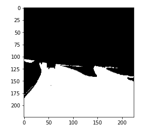
and this is the prediction from the model.
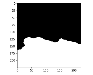
Let’s compare the IOU score for this particular prediction.
# convert predicted mask to flattened numpy array
mask = (output.squeeze() > 0.5).astype(int)
pred = mask.ravel().copy()
# convert ground truth mask to flattened numpy array
gt_mask = gt_mask.cpu().detach().numpy()
target = gt_mask.ravel().copy().astype(int)
# get class indices for Lane
pred_inds = pred == 1
target_inds = target == 1
# calculate intersection
intersection = pred_inds[target_inds].sum()
# calculate union
union = pred_inds.sum() + target_inds.sum() - intersection
# get IoU score
iou = (float(intersection) / float(max(union, 1)))
iou
So the IOU value for this prediction is 0.93. Now, just like we made a prediction on the train set I encourage you that you go ahead and try to take up an image from the validation set and perform the same steps and check the output on the validation set.
Conclusion on Image Segmentation
In this article, we solved the problem of image segmentation in the real-time problem that is lane segmentation. I hope the articles helped you understand how to work with image data, and how to detect lanes from images. We are going to use the same approach, and apply it in a few different domains for example car racing and sports. The next article will discuss solving lane segmentation problems using another deep learning approach.
The learnings are as follows:
1. We are able to find the objects present in the image.
2. We learned to find the specific location of objects in the image.
3. We learned about multiple applications, where image segmentation can be applied.
4. We got to know about different types of image segmentation.
5. We learned to solve the image segmentation.
The media shown in this article is not owned by Analytics Vidhya and is used at the Author’s discretion.


