This article was published as a part of the Data Science Blogathon.
Introduction
Back in 2000, people used to purchase groceries from their local hypermarts. However, in the last 20 years, several online e-commerce stores have been launched. So, instead of going to a physical store, you can visit an online e-commerce store from the comfort of your home. Customers who used to shop from the physical store then started to purchase several products from such e-commerce websites. Also, in 2020, Covid-19 severely impacted the sales of physical hypermarts. This gave the e-commerce demand a boom, and since 2020, more customers have started to shop from such online stores. See the detailed report summary from McKinsey here.
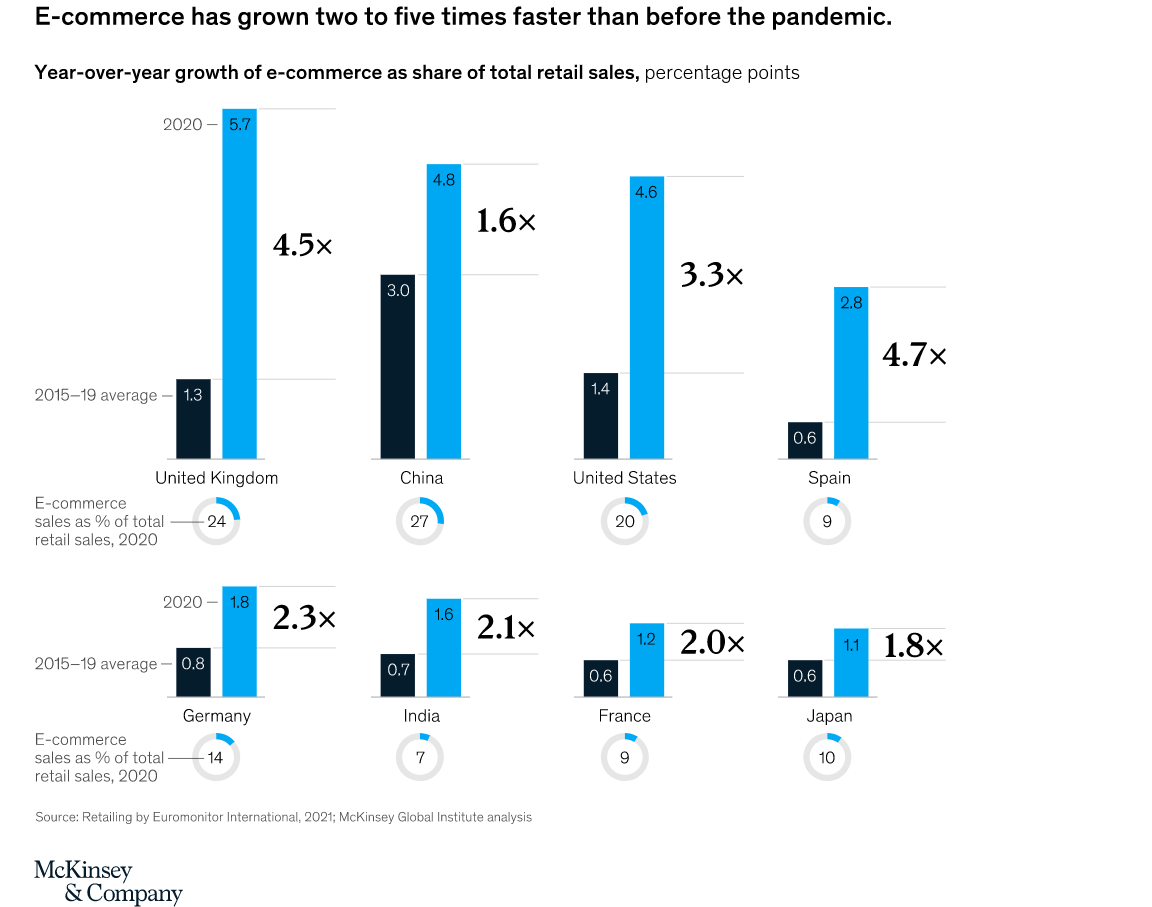
Source: https://www.mckinsey.com/~/media/mckinsey/featured%20insights/future%20of%20organizations/the%20future%20of%20work%20after%20covid%2019/svgz-mgi-covid-fow-ex2.svgz
Many products are available in such e-commerce stores ranging from a toothbrush to a Car. If you want to purchase something, just search for it on the internet, and there will be at least one e-commerce website serving that product. So, many new e-commerce players have been launched in recent years (it has become a very competitive space). In such a competitive space, it is quintessential for the e-commerce store to identify the customer preference and keep a customer interested to shop from their website. This is why the recommendation system helps. A straightforward example would be that if you are purchasing bread, you will possibly purchase butter or Milk. This article will show how to build a recommendation system for Bigbasket.
Importance of Recommendation Systems
Netflix: According to a recent study by McKinsey, Netflix uses personalized recommendations, and it is responsible for 80 percent of the content streamed. This has allowed Netflix to earn 1 billion dollars in a single year. Netflix doesn’t spend much on marketing but on recommendations to improve customer retention.
Amazon: Similarly, 35% of the Amazon website’s sales come from personalized recommendations. So, even Amazon does not spend much on marketing. However, it is still able to retain customers using personalized recommendations.
Source of the above information.
Type of Recommendation System
Popularity Based: Recommends the most popular or most selling products. E.g. Trending videos on Youtube.
Advantages:
- We just need the product information. We don’t need customer preference data.
- We can use this approach for the cold start problem.
Disadvantage: The recommendations are similar for all customers and not personalized.
Content-based: It works on similarities between products. First, we must create a vector representing all the product features. Then, we calculate the similarity between those vectors using methods like:
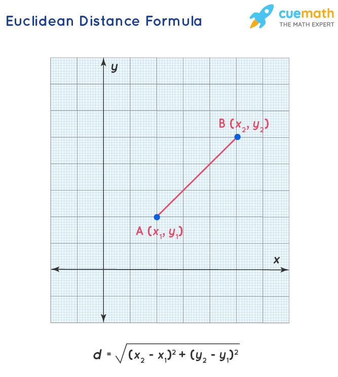
- Euclidean Distance
- Manhattan Distance
- Jaccard Distance
- Cosine Distance (or cosine similarity – we will be using this metric in our article)
For example, if a set of users likes action movies by Jackie Chan, this algorithm may recommend the movies having the below characteristics.
- Having a genre of action
- Having Jackie Chan in the cast.
Advantage: Quick to implement
Disadvantages:
- The recommendations are similar for a set of customers.
- They are slightly personalized based on content.
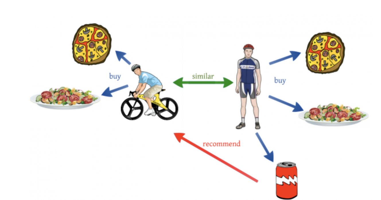
Collaborative-based: It works on similarities between users. If there are 2 users.
Source: https://miro.medium.com/max/1400/1*6_NlX6CJYhtxzRM-t6ywkQ.png
In the illustration above, there are 2 users with similar taste preferences. Both of them liked pie and protein salad and looked like fitness enthusiasts, so they are similar. Now, the user on the right liked a can of energy drink, so we recommend the same energy drink to the user on the left.
Advantages: It gives personalized recommendations for each user basis their historic preferences.
Disadvantage: The algorithm needs a lot of historical data to train, and the model’s accuracy increases with increased data.
Hybrid: Here, we combine all the above 3 recommender systems.
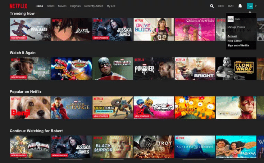
For example, the Netflix homepage has several strips for recommending content to its subscriber.
- It has strips like
- Trending now
- Popular on Netflix
- Watch it again
- Personalized recommendation for the subscriber
What is Bigbasket?

Bigbasket is one of the biggest online grocery stores in India. It was launched in 2011, and several competitors have challenged it for market share. However, it can still retain its fair share in the market.
Understand the Data for Recommendation System
We will be using a publicly available dataset from Kaggle. It can be downloaded from here
About this file. This dataset contains the below 10 columns:
- index – the serial number
- product – Title (or name) of the product
- category – Category of the product
- sub_category – Subcategory of the product
- brand – Brand of the product
- sale_price – Price at which product is being sold on the site
- market_price – The market price of the product
- type – Type into which product falls
- rating – aggregate product rating (out of 5) by customers
- description – Description of the product
Import Relevant Libraries
Python Code:
#Basic Libraries
import numpy as np
import pandas as pd
#Visualization Libraries
import matplotlib.pyplot as plt
import seaborn as sns
import plotly.express as px
#Text Handling Libraries
import re
from sklearn.feature_extraction.text CountVectorizer
from sklearn.metrics.pairwise import cosine_similarity
import pandas as pd
df = pd.read_csv('BigBasket Products.csv',index_col='index')
print(df.shape)
print(df.head())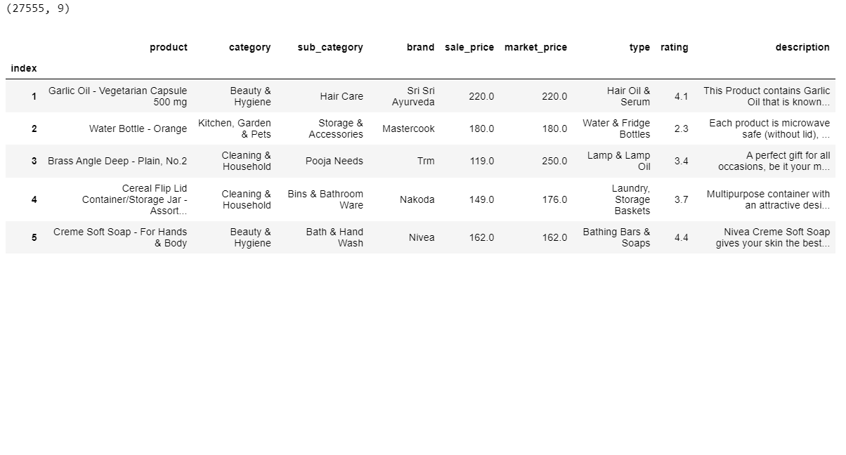
EDA (Exploratory Data Analysis) and Data Cleaning
“I can’t make bricks without clay.” ― Arthur Conan Doyle.
We need data to make our recommendation system model. So, EDA is crucial because it allows us to understand the data. Around 70-80% of the time is spent in this step. There may be several issues with data. We need to spend time here and get introduced to the data.
Check for Missing data: If the data is null or missing, we cannot use it for data analysis. So, let’s look at the data distribution.
Missing count:
print('Null Data Count In Each Column')
print('-'*30)
print(df.isnull().sum())
print('-'*30)
print('Null Data % In Each Column')
print('-'*30)
for col in df.columns:
    null_count = df[col].isnull().sum()
    total_count = df.shape[0]
    print("{} : {:.2f}".format(col,null_count/total_count * 100))
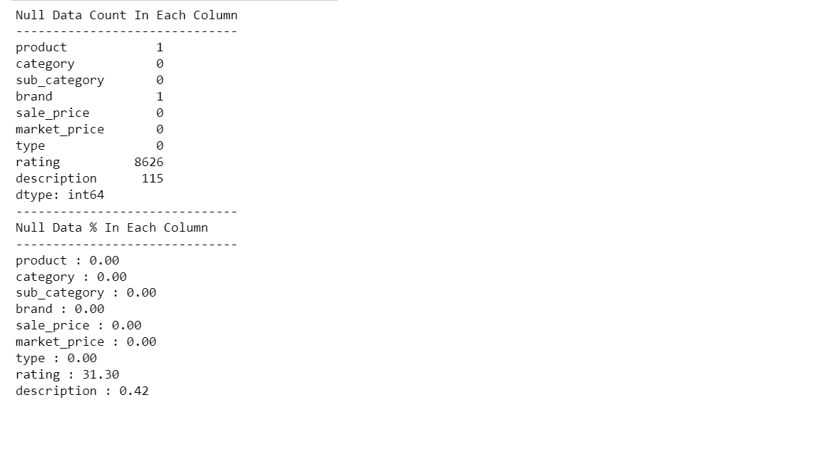
Findings from the EDA:
- There is a product without a name.
- There is a product without a brand.
- 115 products do not have a description.
- 8626 products do not have ratings.
The above features are important for building a recommendation system. So, we will drop the rows from data that contain missing values.
Python code:
df = df.dropna()
print(df.shape)
Output :
(18840, 9)
Even after dropping nulls, we have a good data size of 18840 records.
Understanding Data Types of Columns
df.dtypes
Output:
product          object
category         object
sub_category     object
brand            object
sale_price      float64
market_price    float64
type             object
rating          float64
description      object
Findings from this step:
The features sale_price, market_price, and rating are numeric (as they are represented using float64). The rest are all string features (represented as objects).
Univariate Analysis in Recommendation System
Here, we will understand the data distribution of several columns. A look at category column distribution
counts = df['category'].value_counts()
count_percentage = df['category'].value_counts(1)*100
counts_df = pd.DataFrame({'Category':counts.index,'Counts':counts.values,'Percent':np.round(count_percentage.values,2)})
display(counts_df)
px.bar(data_frame=counts_df,
 x='Category',
 y='Counts',
 color='Counts',
 color_continuous_scale='blues',
 text_auto=True,
 title=f'Count of Items in Each Category')
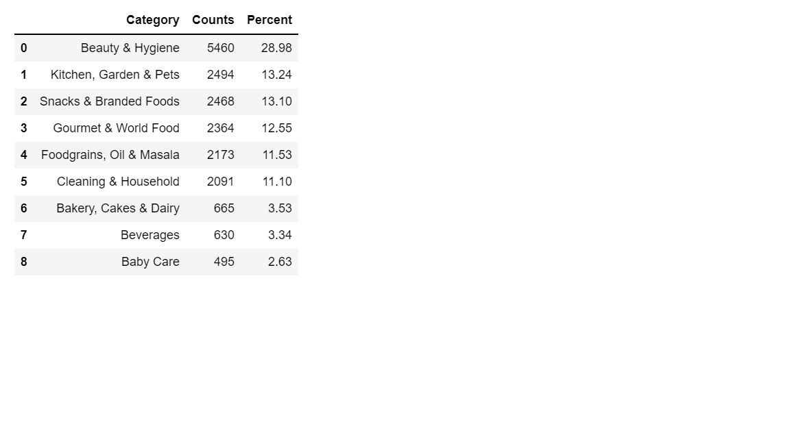
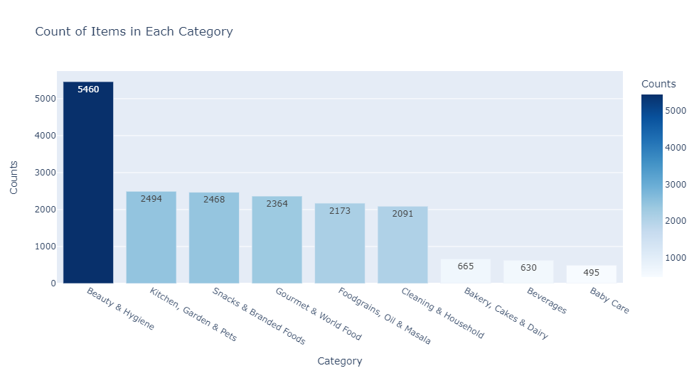
Findings:
- Beauty and Hygiene have a total of 5460 products. It covers 28.98% of the total product portfolio.
- Next, the best category is Kitchen, Garden, and Pets, which has 2494 products. It covers 13.24% of the total product portfolio.
- Baby care has the lowest product count of 495 products. It covers 2.63% of the total product portfolio.
A look at sub_category column distribution
counts = df['sub_category'].value_counts()
count_percentage = df['sub_category'].value_counts(1)*100
counts_df = pd.DataFrame({'sub_category':counts.index,'Counts':counts.values,'Percent':np.round(count_percentage.values,2)})
print('unique sub_category values',df['sub_category'].nunique())
print('Top 10 sub_category')
display(counts_df.head(10))
print('Bottom 10 sub_category')
display(counts_df.tail(10))
px.bar(data_frame=counts_df[:10],
x='sub_category',
y='Counts',
color='Counts',
color_continuous_scale='blues',
text_auto=True,
title=f'Top 10 Bought Sub_Categories')
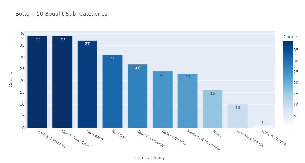
px.bar(data_frame=counts_df[-10:],
x='sub_category',
y='Counts',
color='Counts',
color_continuous_scale='blues',
text_auto=True,
title=f'Bottom 10 Bought Sub_Categories')
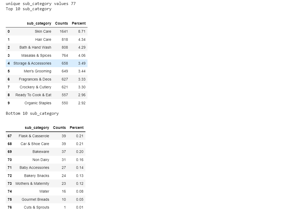
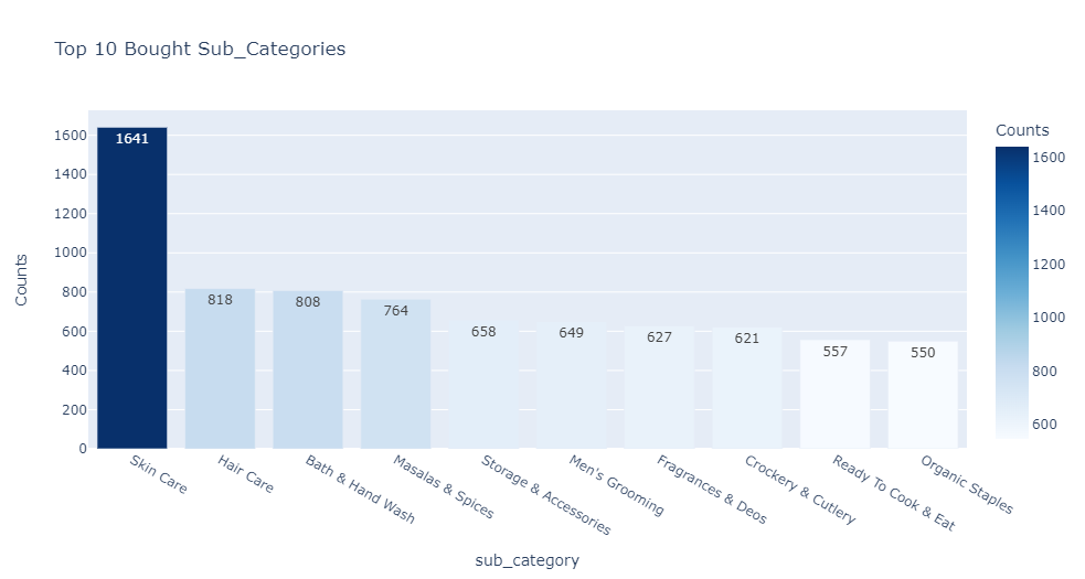
Findings:
- There are 77 unique sub_category values.
- Skin Care has a total of 1641 products. It covers 8.71% of the total product portfolio.
- The next best sub_category is Hair Care which has a total of 818 products. It covers 4.34% of the total product portfolio.
- Cuts & Sprouts has the lowest product count of 1 product. It barely covers 0.01% of the total product portfolio.
A look at brand column distribution
column = 'brand'
counts = df[column].value_counts()
count_percentage = df[column].value_counts(1)*100
counts_df = pd.DataFrame({column:counts.index,'Counts':counts.values,'Percent':np.round(count_percentage.values,2)})
print('unique '+str(column)+' values',df['sub_category'].nunique())
print('Top 10 '+str(column))
display(counts_df.head(10))
print('Bottom 10 '+str(column))
display(counts_df.tail(10))
px.bar(data_frame=counts_df.head(10),
 x=column,
 y='Counts',
 color='Counts',
 color_continuous_scale='blues',
 text_auto=True,
 title=f'Top 10 Brand Items based on Item Counts')
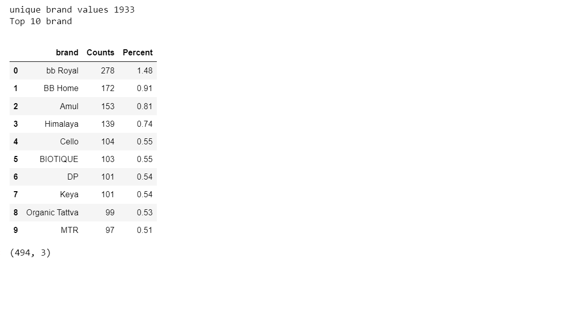
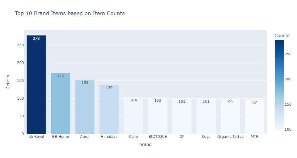
Findings:
- There are 1933 unique values for brands.
- There are 494 brands having a single product.
- The top 2 brands are of BigBasket.
- bb Royal has a total of 278 products. It covers 1.48% of the total product portfolio.
- The next best brand is BB Home, which has 172 products. It covers 0.91% of the total product portfolio.
A look at type column distribution
column = 'type'
counts = df[column].value_counts()
count_percentage = df[column].value_counts(1)*100
counts_df = pd.DataFrame({column:counts.index,'Counts':counts.values,'Percent':np.round(count_percentage.values,2)})
print('unique '+str(column)+' values',df[column].nunique())
print('Top 10 '+str(column))
display(counts_df.head(10))
counts_df[counts_df['Counts']==1].shape
px.bar(data_frame=counts_df.head(10),
 x='type',
 y='Counts',
 color='Counts',
 color_continuous_scale='blues',
 text_auto=True,
 title=f'Top 10 Types of Products based on Item Counts')
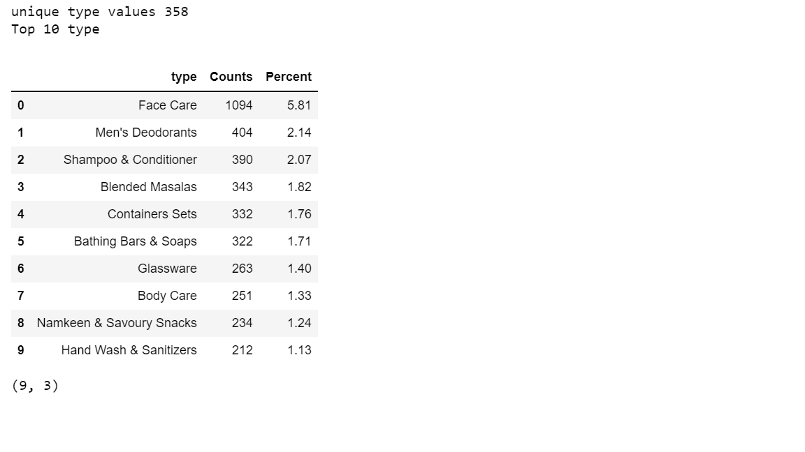
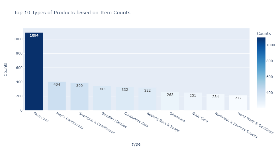
Findings:
- There are 358 unique values for type.
- There are 9 types having a single product.
- Face Care has a total of 1094 products. It covers 5.81% of the total product portfolio.
- Next, the best type is Men’s Deodorant, which has 404 products. It covers 2.14% of the total product portfolio.
Ratings Analysis
Since this is a numeric column, Let’s look at the histogram of this column.
print(df['rating'].describe())
df['rating'].hist(bins=10)
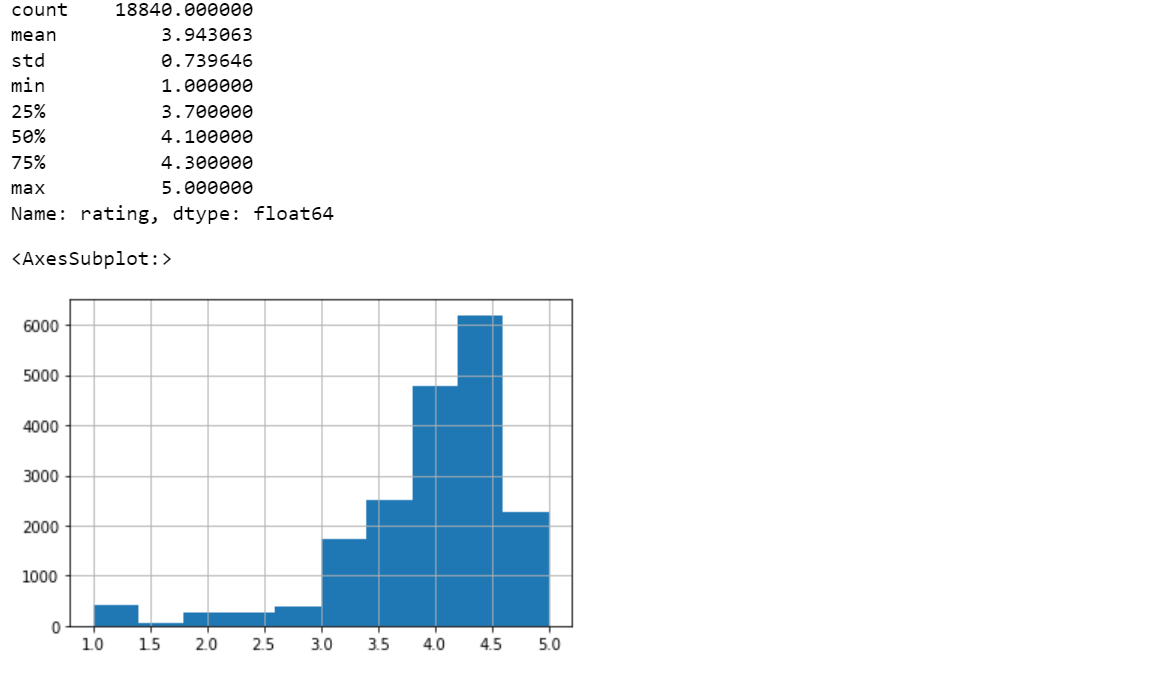
We can see that histogram is skewed towards the right, which means that most of the products have a higher rating.
How many Ratings are between the interval of 0 to 1, 1 to 2, and so on?
pd.cut(df.rating,bins = [0,1,2,3,4,5]).reset_index().groupby(['rating']).size()
Output:
rating
(0, 1]      387
(1, 2]      335
(2, 3]     1347
(3, 4]     6559
(4, 5]    10212
Findings:
- 10212 products had a rating between 4 and 5.
- 387 products had a rating between 0 and 1.
Feature Engineering for Recommendation System
Here, we can create new features which can improve the recommendations. We have the sale_price and market_price. Let’s create a feature discount%
Formula = [ (market_price – sale_price)/sale_price ] * 100
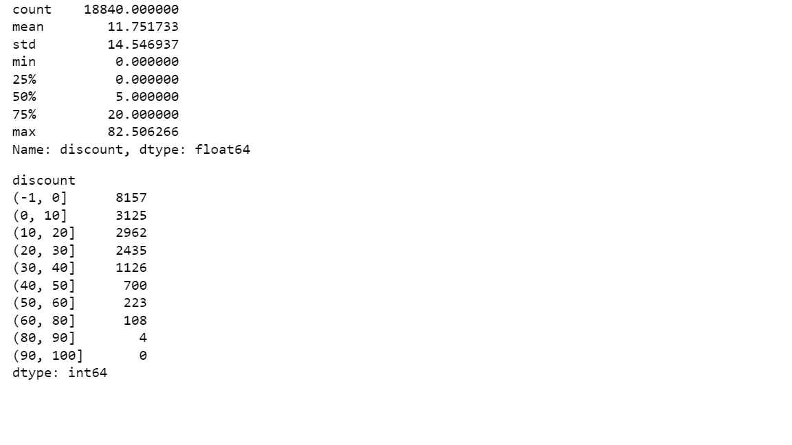
df['discount'] = (df['market_price']-df['sale_price'])*100/df['market_price']
print(df['discount'].describe())
pd.cut(df.discount,bins = [-1,0,10,20,30,40,50,60,80,90,100]).reset_index().groupby(['discount']).size()
Since this is a numeric column, Let’s look at the histogram of this column.
df['discount'].hist()
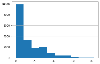
Findings:
- 8157 products do not have any discount.
- At least 4 products have above 80% discount.
Bivariate Analysis
Is there any relation between rating and discount?
ax = df.plot.scatter(x='rating',y='discount')
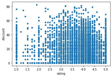
Findings: Looking at the scatter plot, we do not see any association between rating and discount.
Let’s Clean a Few String Columns
The category column contains ‘Kitchen, Garden & Pets.’ We will clean it, so it contains [kitchen, garden, pets]. A similar transformation will be applied to sub_category, type, and brand features.
Now, let’s create one feature (product_classification_features) which appends all the above 4 cleaned columns.
df2 = df.copy()
rmv_spc = lambda a:a.strip()
get_list = lambda a:list(map(rmv_spc,re.split('& |, |*|n', a)))
for col in ['category', 'sub_category', 'type']:
    df2[col] = df2[col].apply(get_list)
def cleaner(x):
    if isinstance(x, list):
        return [str.lower(i.replace(" ", "")) for i in x]
    else:
        if isinstance(x, str):
            return str.lower(x.replace(" ", ""))
        else:
            return ''
for col in ['category', 'sub_category', 'type','brand']:
    df2[col] = df2[col].apply(cleaner)
def couple(x):
    return ' '.join(x['category']) + ' ' + ' '.join(x['sub_category']) + ' '+x['brand']+' ' +' '.join( x['type'])
df2['product_classification_features'] = df2.apply(couple, axis=1)
Now, we have the data ready. Let us build a simple logic for recommendations based on popularity. We will use the recommender feed – type, category, or sub_category. It will return the most popular product or the product having the highest rating.
def recommend_most_popular(col,col_value,top_n=5):
return df[df[col]==col_value].sort_values(by=’rating’,ascending = False).head(top_n)[[‘product’,col,’rating’]]
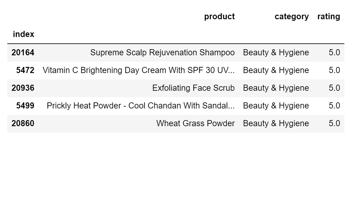
Let’s look at the most popular products for the category = Beauty & Hygiene
recommend_most_popular(col='category',col_value='Beauty & Hygiene')
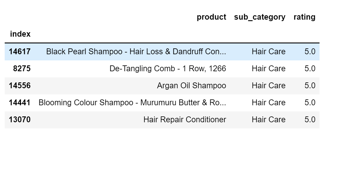
Let’s look at the most popular products for sub_category = Hair Care
recommend_most_popular(col='sub_category',col_value='Hair Care')
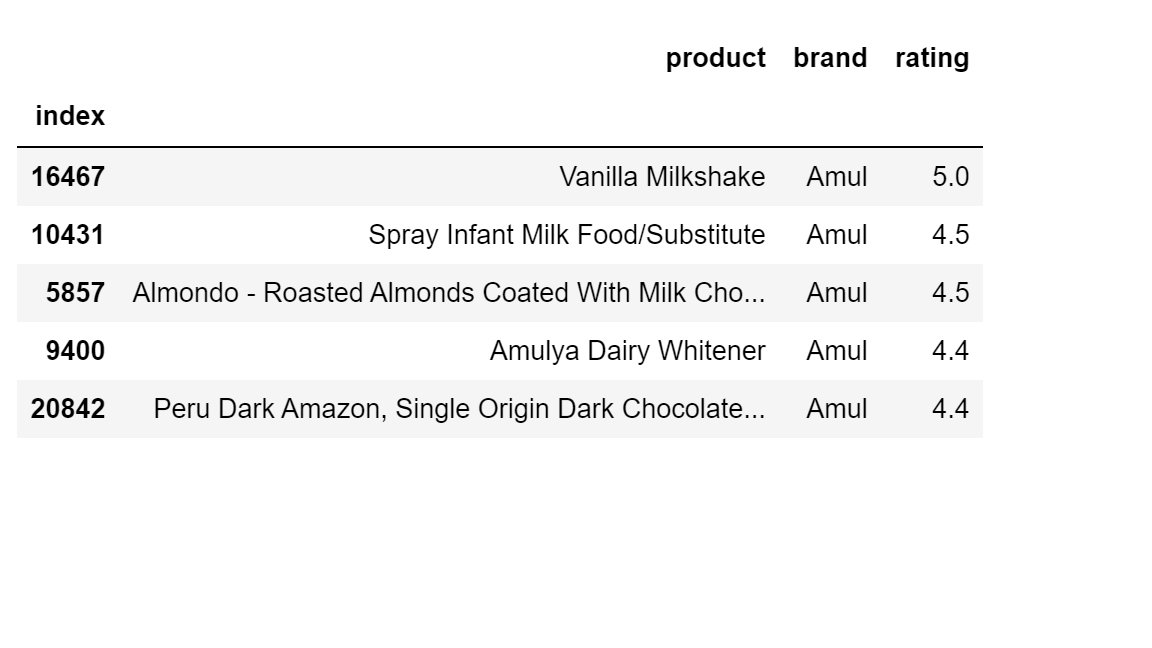
Let’s look at the most popular products for the brand = Amul
recommend_most_popular(col='brand',col_value='Amul')
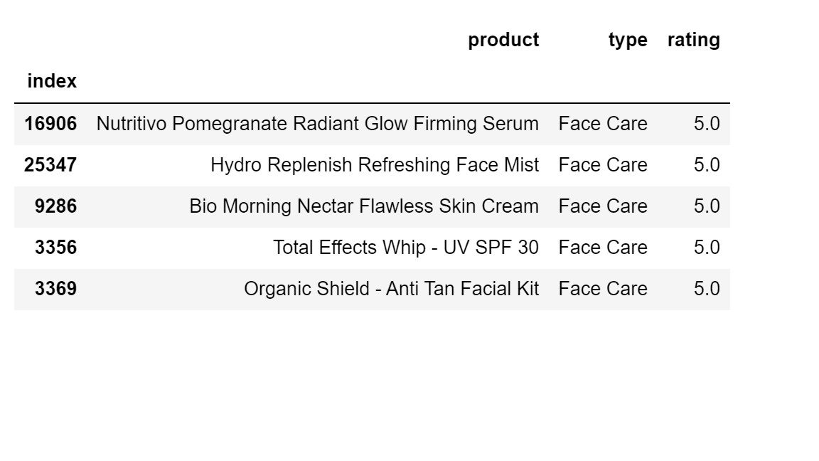
Let’s look at the most popular products for type = Face Care
recommend_most_popular(col='type',col_value='Face Care')
Let’s Build a Content-based Recommendation System
As the name suggests, these algorithms use the data of the product we want to recommend. E.g., Kids like Toy Story 1 movies. Toy Story is an animated movie created by Pixar studios – so the system can recommend other animated movies by Pixar studios like Toy Story 2. For our, e.g., we will use the product metadata like category, sub_category, type, price, etc. We will extract similar products from the product portfolio based on these features. The feature we created earlier (product_classification_features) will be helpful here.
We will use CountVectorizer to create a feature space.
e.g., You have 3 sentences:
s1 = ‘Ram is a boy
s2 = ‘Ram is good
s3 = ‘Good is that boy.’
So, we first convert them into lowercase
s1 = ‘ram is boy’
s2 = ‘ram is good’
s3 = ‘good is that boy’
So, Vocabulary consists of {‘boy’, ‘good’, ‘is’, ‘ram’, ‘that’} as unique words.
So, when you use CountVectorizer, it creates 5 features, each representing the count of occurrence of that word.
from sklearn.feature_extraction.text import CountVectorizer
from scipy.spatial import distance
vectorizer = CountVectorizer(lowercase=True)
X = vectorizer.fit_transform([s1,s2,s3])
X.toarray()
count_vect_df = pd.DataFrame(X.toarray(),columns=vectorizer.get_feature_names_out())
count_vect_df
| boy | good | is | ram | that | |
|---|---|---|---|---|---|
| 0 | 1 | 0 | 1 | 1 | 0 |
| 1 | 0 | 1 | 1 | 1 | 0 |
| 2 | 1 | 1 | 1 | 0 | 1 |
Once we have these vectors, we can use the below similarity metrics for identifying and recommending similar products
1. Euclidean Distance: It measures the straight line distance between the 2 vectors.

For our example, Euclidean Distance looks like the below:
distance.cdist(count_vect_df, count_vect_df, metric='euclidean').round(2)
Output
array([[0.  , 1.  , 1.73],
       [1.  , 0.  , 1.41],
       [1.73, 1.41, 0.  ]])
In the above example, all diagonal entries are 0, which is intuitive – each sentence’s Euclidean Distance is 0. Also, Euclidean Distance between
- s1 and s2 = 1
- s2 and s3 = 1.41
- s1 and s3 = 1.73
So, s1 is closer to s2
s2 is closer to s1
s3 is closer to s2
Manhattan Distance: It measures the absolute differences between the two vectors.
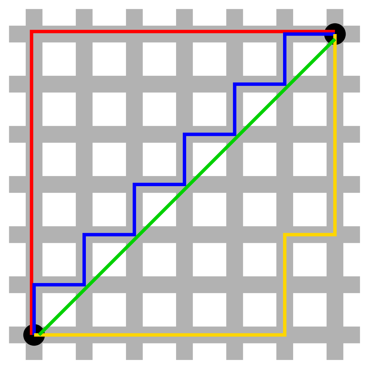
- The green line represents Euclidean distance.
- The red, blue, and yellow lines represent Manhattan distance.
- It is a vehicle’s travel route to reach from one location to another.
For our example, Manhattan Distance looks like the below:
distance.cdist(count_vect_df, count_vect_df, metric='cityblock').astype('int')
Output
array([[0, 2, 3],
       [2, 0, 3],
       [3, 3, 0]])
In the above example, all diagonal entries are 0, which is intuitive – the Manhattan Distance of each sentence with itself is 0. Also, Manhattan Distance between
- s1 and s2 = 2
- s2 and s3 = 3
- s1 and s3 = 3
So, s1 is closer to s2
s2 is closer to s1
s3 is equidistant from s2 and s1
Jaccard Distance: It measures the ratio of common words between 2 sentences to the overall unique words in those 2 sentences.
For s1 and s2, it is calculated as
s1 and s2 = len({‘is’,’ram’})/len({‘boy’,’is’,’ram’,’good’}) = 0.5
For our example, Jaccard Distance looks like the below:
distance.cdist(count_vect_df, count_vect_df, metric='jaccard').astype('int')
Output:
array([[0. , 0.5, 0.6],
       [0.5, 0. , 0.6],
       [0.6, 0.6, 0. ]])
So, Jaccard’s distance between
- s1 and s2 = 0.5
- s2 and s3 = 0.6
- s1 and s3 = 0.6
So, s1 is closer to s2
s2 is closer to s1
s3 is equidistant from s2 and s1
Cosine Distance (or cosine similarity – we will be using this metric in our article) we will use cosine similarity for identifying and recommending similar products.
Cosine similarity measures the angle between the 2 vectors.
Cosine similarity can give a value between -1 to +1. A value of -1 means that the products are opposite or non-similar and a value of +1 means that the 2 products are the same.
Cosine similarity looks like below:
Cosine similarity is 1- cosine distance
1-distance.cdist(count_vect_df, count_vect_df, metric='cosine').round(2)
Output:
array([[1.  , 0.67, 0.58],
       [0.67, 1.  , 0.58],
       [0.58, 0.58, 1.  ]])
In the above example, all diagonal entries are 1, which is intuitive – each sentence’s cosine similarity is 1.
Also, cosine similarity between
- s1 and s2 = 0.67
- s2 and s3 = 0.58
- s1 and s3 = 0.58
So, s1 is closer to s2
s2 is closer to s1
s3 is equidistant from s2 and s1
Let’s calculate the cosine similarity of the product_classification_features for all the products.
count = CountVectorizer(stop_words='english')
count_matrix = count.fit_transform(df2['product_classification_features'])
cosine_sim = cosine_similarity(count_matrix, count_matrix)
cosine_sim_df = pd.DataFrame(cosine_sim)
The above matrix contains the cosine similarity of each product vs the rest of the products in catalog. Let’s build a recommender using cosine similarity
def content_recommendation_v1(title):
    a = df2.copy().reset_index().drop('index',axis=1)
    index = a[a['product']==title].index[0]
    top_n_index = list(cosine_sim_df[index].nlargest(10).index)
    try:
        top_n_index.remove(index)
    except:
        pass
    similar_df = a.iloc[top_n_index][['product']]
    similar_df['cosine_similarity'] = cosine_sim_df[index].iloc[top_n_index]
    return similar_df
Let’s see the recommendations for a few products.
title = 'Water Bottle - Orange'
content_recommendation_v1(title)
Output:
| product | cosine_similarity | |
|---|---|---|
| 109 | Glass Water Bottle – Aquaria Organic Purple | 0.875 |
| 705 | Glass Water Bottle With Round Base – Transparent… | 0.875 |
| 1155 | H2O Unbreakable Water Bottle – Pink | 0.875 |
| 1500 | Water Bottle H2O Purple | 0.875 |
| 1828 | H2O Unbreakable Water Bottle – Green | 0.875 |
| 1976 | Regel Tritan Plastic Sports Water Bottle – Black | 0.875 |
| 2182 | Apsara 1 Water Bottle – Assorted Colour | 0.875 |
| 2361 | Glass Water Bottle With Round Base – Yellow, B… | 0.875 |
| 2485 | Trendy Stainless Steel Bottle With Steel Cap -… | 0.875 |
Findings:
- In this example, we can recommend bottles. However, we are recommending all the colors.
- Also, the cosine similarity is the same for all the recommendations.
title = 'Dark Chocolate- 55% Rich In Cocoa'
content_recommendation_v1(title)
Output:
| product | cosine_similarity | |
|---|---|---|
| 105 | I Love You Fruit N Nut Chocolate | 1.0 |
| 1144 | Choco Cracker – Magical Crystal With Milk Choc… | 1.0 |
| 1718 | Dark Chocolate – Single Origin, India | 1.0 |
| 2517 | Fruit N Nut, Dark Chocolate- 55% Rich In Cocoa | 1.0 |
| 3117 | Colombia Classique Black, Single Origin Dark C… | 1.0 |
| 3167 | Dark Chocolate | 1.0 |
| 4013 | Almondo – Roasted Almonds Coated With Milk Cho… | 1.0 |
| 4358 | Sugar-Free Dark Chocolate | 1.0 |
| 5867 | Milk Compound Slab – MCO-11 | 1.0 |
Findings:
- In this example, we can recommend all types of Chocolates.
- However, the top recommendation should be dark chocolate.
- Also, the cosine similarity is the same for all the recommendations.
Improving the Model
Let us tweak the algorithm. Let us also use the product column to create another cosine similarity. We will take the average of both the cosine similarity and see if the results are better.
count2 = CountVectorizer(stop_words='english',lowercase=True)
count_matrix2 = count2.fit_transform(df2['product'])
cosine_sim2 = cosine_similarity(count_matrix2, count_matrix2)
cosine_sim_df2 = pd.DataFrame(cosine_sim2)
def content_recommendation_v2(title):
    a = df2.copy().reset_index().drop('index',axis=1)
    index = a[a['product']==title].index[0]
    similar_basis_metric_1 = cosine_sim_df[cosine_sim_df[index]>0][index].reset_index().rename(columns={index:'sim_1'})
    similar_basis_metric_2 = cosine_sim_df2[cosine_sim_df2[index]>0][index].reset_index().rename(columns={index:'sim_2'})
    similar_df = similar_basis_metric_1.merge(similar_basis_metric_2,how='left').merge(a[['product']].reset_index(),how='left')
    similar_df['sim'] = similar_df[['sim_1','sim_2']].fillna(0).mean(axis=1)
    similar_df = similar_df[similar_df['index']!=index].sort_values(by='sim',ascending=False)
    return similar_df[['product','sim']].head(10)
title = 'Water Bottle - Orange'
content_recommendation_v2(title)
Output:
| product | sim | |
|---|---|---|
| 669 | Sante Infuser Water Bottle – Orange | 0.824798 |
| 2024 | H2o Unbreakable Water Bottle – Orange | 0.824798 |
| 2565 | Swat Pet Water Bottle – Orange | 0.824798 |
| 1912 | Glass Water Bottle – Circo Orange & Lemon | 0.791053 |
| 2084 | Spray Glass water Bottle With Cork – Orange | 0.791053 |
| 1924 | Sip-It-Plastic Water Bottle | 0.726175 |
| 1997 | Water Bottle – Twisty, Pink | 0.726175 |
| 1290 | Plastic Water Bottle – Pink | 0.726175 |
| 195 | Water Bottle H2O Purple | 0.726175 |
| 1863 | Water Bottle – Apsara 1 Assorted Colour | 0.695699 |
Findings: The results are much better for this. The orange color bottles have a higher similarity.
title = 'Dark Chocolate- 55% Rich In Cocoa'
content_recommendation_v2(title)
Output:
| product | sim | |
|---|---|---|
| 437 | Fruit N Nut, Dark Chocolate- 55% Rich In Cocoa | 0.922577 |
| 2340 | Sugar-Free Dark Chocolate- 55% Rich In Cocoa | 0.922577 |
| 2717 | Rich Cocoa Dark Chocolate Bar | 0.837500 |
| 561 | Dark Chocolate | 0.816228 |
| 504 | Dlite Rich Cocoa Dark Chocolate Bar | 0.802648 |
| 3137 | Bitter Chocolate- 75% Rich In Cocoa | 0.800000 |
| 2544 | Peru Dark Amazon, Single Origin Dark Chocolate… | 0.782843 |
| 3148 | Bournville Rich Cocoa 70% Dark Chocolate Bar | 0.775562 |
| 548 | Colombia Classique Black, Single Origin Dark C… | 0.769680 |
| 2941 | Tanzania Chocolat Noir, Single Origin Dark Cho… | 0.769680 |
Findings: Even here, we see Dark chocolate products having higher similarities.
Let us run the recommendation for a few more products.
title = 'Nacho Round Chips'
content_recommendation_v2(title)
Output:
| product | sim | |
|---|---|---|
| 3766 | Nacho Chips – Crunchy Pizza | 0.788675 |
| 718 | Nacho Chips – Jalapeno | 0.770833 |
| 3630 | Nacho Chips – Cheese | 0.770833 |
| 1680 | Nacho Chips – Salsa | 0.770833 |
| 464 | Nacho Chips – Peri Peri | 0.735702 |
| 3140 | Nacho Chips – Sweet Chilli | 0.726175 |
| 3912 | Nacho Chips – Roasted Masala | 0.726175 |
| 4478 | Nacho Chips – Jalapeno, No Onion, No Garlic | 0.695699 |
| 1233 | Nacho Chips – Peri Peri | 0.673202 |
| 86 | Nacho Chips – Cheese With Herbs, No Onion, No … | 0.673202 |
title = 'Chewy Mints - Lemon'
content_recommendation_v2(title)
Output:
| product | sim | |
|---|---|---|
| 452 | Chewy Candy Stick – Strawberry Flavour | 0.557671 |
| 324 | Orbit Sugar-Free Chewing Gum – Lemon & Lime | 0.537680 |
| 1558 | Chewy Mints – Spearmint Flavour Candy | 0.525460 |
| 711 | Chewing Gum – Peppermint | 0.500000 |
| 2676 | Chewing Gum – Peppermint | 0.500000 |
| 1734 | Chewing Gum – Peppermint | 0.500000 |
| 2842 | Orange Chewy Dragees | 0.433928 |
| 877 | Sugarfree Strawberry | 0.428571 |
| 1063 | White Xylitol Sugarfree Spearmint Flavour Chew… | 0.428571 |
| 1543 | Mint – Sugarfree, Peppermint Flavour | 0.428571 |
title = 'Veggie - Fingers'
content_recommendation_v2(title)
Output:
| product | sim | |
|---|---|---|
| 1186 | Veggie Fingers – Veggie Delight with Corn, Car… | 0.853553 |
| 980 | Veggie – Nuggets | 0.750000 |
| 814 | Veggie Burger Patty | 0.704124 |
| 2639 | Veggie – Nuggets | 0.687500 |
| 331 | Veggie Stix | 0.687500 |
| 2656 | Veggie Pizza Pocket | 0.641624 |
| 840 | Veggie Burger Patty | 0.641624 |
| 1231 | Crispy Veggie Burger Patty | 0.614277 |
| 1082 | Chicken Fingers – Garlic | 0.557678 |
| 1121 | Quick Snack – Fish Fingers | 0.530330 |
The recommendation results look relevant.
Kudos on building your content recommendation system using NLP.
Conclusion
Companies like Amazon and Netflix can drive a lot of revenue using a recommendation system. They can engage and retain existing customers by recommending relevant content to them. In this article, we saw different types of recommendation systems. We then used a publicly available dataset, did a thorough EDA, and developed a content-based recommendation system. There are several metrics we can use to identify similarities between products. We used cosine similarity for our recommendation system.
Key takeaways:
- For a cold start problem, we should use Popularity Based recommendation system. Recommends the most popular or most selling products. This gives generic recommendations to all users.
- We can use a content-based recommendation system if we want to recommend similar products to a set of users.
- Once we have a good amount of user preference data, we can build Collaborative-based recommendations. Here, we give a personalized recommendation to each user.
I hope you liked this guide on building content recommendations. Share your feedback with me in the comments section below.
Feel free to connect with me on LinkedIn if you want to discuss this with me.
The media shown in this article is not owned by Analytics Vidhya and is used at the Author’s discretion.
Data Scientist with extensive experience in solving many real world business problems across different domains. Possess fine blend of business knowledge, maths/stats and technology/programming.
Experienced in handling client facing roles, stakeholder management, effective communication with presentation & negotiation skills.


Thank you for sharing this informative post on building a content-based recommendation system! As technology continues to advance, it's important to understand and keep up with the latest developments in recommendation systems.
While executing below code, getting error message it says , nothing to repeat at position 6, Position 6 refering to "for col in ['category', 'sub_category', 'type']:" Code: get_list = lambda a:list(map(rmv_spc,re.split('& |, |*|n', a))) for col in ['category', 'sub_category', 'type']: df2[col] = df2[col].apply(get_list) Could you please help on this ?