Image processing is a widely used concept to exploit the information from the images. Image processing algorithms take a long time to process the data because of the large images and the amount of information available in it. So, in these edge-cutting techniques, it is necessary to reduce the amount of information that the algorithm should focus on. Sometimes this could be done only by passing the edges of the image. So in this blog let’s understand the Canny edge detector and Holistically Nested Edge Detector.
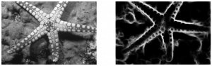
An edge in an image is a significant local change in the image intensity. As the name suggests, edge detection is the process of detecting the edges in an image. The example below depicts an edge detection of a starfish’s image.
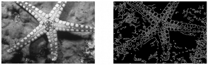
Fig 1.1 Edge Detection
Discontinuities in depth, surface orientation, scene illumination variations, and material properties changes lead to discontinuities in image brightness. We get the set of curves that indicate the boundaries of objects and surface markings, and curves that correspond to discontinuities in surface orientation.
Thus, applying an edge detection algorithm to an image may significantly reduce the amount of data to be processed and may therefore filter out information that may be regarded as less relevant while preserving the important structural properties of an image.
As you can see in fig 1.1, the structural properties of an image are captured through edge detection.
Having discussed the importance of Edge Detection Algorithms, this section will focus on understanding some of the popular and widely used edge detection algorithms.
There are multiple approaches for edge detection. Let us broadly divide the approaches into-
In the conventional approach, we have discussed filter-based approaches such as Sobel and Prewitt filters in our previous article. Now, let us discuss one of the most popular edge detection algorithms – The canny edge detector, and compare it with Sobel and Prewitt.
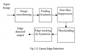
The Canny Edge Detection algorithm is a widely used edge detection algorithm in today’s image processing applications. It works in multiple stages as shown in fig 1.2. Canny edge detection algorithm produces smoother, thinner, and cleaner images than Sobel and Prewitt filters.
Here is a summary of the canny edge detection algorithm-
The input image is smoothened, Sobel filter is applied to detect the edges of the image. Then we apply non-max suppression where the local maximum pixels in the gradient direction are retained, and the rest are suppressed. We apply thresholding to remove pixels below a certain threshold and retain the pixels above a certain threshold to remove edges that could be formed due to noise. Later we apply hysteresis tracking to make a pixel strong if any of the 8 neighboring pixels are strong.
Now, we will discuss each step in detail.
There are 5 steps involved in Canny edge detection, as shown in fig 1.2 above. We will be using the following image for illustration.
In this step, we convert the image to grayscale as edge detection does not dependent on colors. Then we remove the noise in the image with a Gaussian filter as edge detection is prone to noise.
We then apply the Sobel kernel in horizontal and vertical directions to get the first derivative in the horizontal direction (Gx) and vertical direction (Gy) on the smoothened image. We then calculate the edge gradient(G) and Angle(θ) as given below,
Edge_Gradient(G) = √(Gx2+Gy2)
Angle(θ)=tan-1(Gy/Gx)
We know that the gradient direction is perpendicular to the edge. We round the angle to one of four angles representing vertical, horizontal, and two diagonal directions.
Now we remove all the unwanted pixels which may not constitute the edge. For this, every pixel is checked in the direction of the gradient if it is a local maximum in its neighbourhood. If it is a local maximum, it is considered for the next stage, otherwise, it is darkened with 0. This will give a thin line in the output image.
Pixels due to noise and color variation would persist in the image. So, to remove this, we get two thresholds from the user, lowerVal and upperVal. We filter out edge pixels with a weak gradient(lowerVal) value and preserve edge pixels with a high gradient value(upperVal). Edges with an intensity gradient more than upperVal are sure to edge, and those below lowerVal are sure to be non-edges, so discarded. The pixels that have pixel value lesser than the upperVal and greater than the lowerVal are considered part of the edge if it is connected to a “sure-edge”. Otherwise, they are also discarded.
A pixel is made as a strong pixel if either of the 8 pixels around it is strong(pixel value=255) else it is made as 0. 
That’s pretty much about Canny Edge Detection. As you can see here, the edges are detected from an image.
Now, we will explore the deep learning-based approaches for edge detection. But why do we need to go for the Deep Learning based edge detection algorithms in the first place? Canny edge detection focuses only on local changes, and it does not understand the image’s semantics, i.e., the content. Hence, Deep Learning based algorithms are proposed to solve these problems. We will discuss it in detail now.
But before we dive into the math of Deep learning, let us first try to implement the canny edge detector and the deep learning-based model(HED) in OpenCV.
Let us import the necessary modules
import cv2 from skimage.metrics import mean_squared_error,peak_signal_noise_ratio,structural_similarity
import matplotlib.pyplot as plt
The following code applies a canny edge detector on an image of starfish
img_path = 'starfish.png'
#Reading the image
image = cv2.imread(img_path)
(H, W) = image.shape[:2]
# convert the image to grayscale
gray = cv2.cvtColor(image, cv2.COLOR_BGR2GRAY)
# blur the image
blurred = cv2.GaussianBlur(gray, (5, 5), 0)
# Perform the canny operator
canny = cv2.Canny(blurred, 30, 150)
Let’s see the output of the canny edge detector
fig,ax =  plt.subplots(1,2,figsize=(18, 18))
ax[0].imshow(gray,cmap='gray')
ax[1].imshow(canny,cmap='gray')
ax[0].axis('off')
ax[1].axis('off')
Next, let us jump into the code of HED before going to the math of it.
#This class helps in cropping the specified coordinated in the function
class CropLayer(object):
    def __init__(self, params, blobs):
        # initialize our starting and ending (x, y)-coordinates of
        self.startX = 0
        self.startY = 0
        self.endX = 0
        self.endY = 0
    def getMemoryShapes(self, inputs):
        (inputShape, targetShape) = (inputs[0], inputs[1])
        (batchSize, numChannels) = (inputShape[0], inputShape[1])
        (H, W) = (targetShape[2], targetShape[3])
        # compute the starting and ending crop coordinates
        self.startX = int((inputShape[3] - targetShape[3]) / 2)
        self.startY = int((inputShape[2] - targetShape[2]) / 2)
        self.endX = self.startX + W
        self.endY = self.startY + H
        # return the shape of the volume (we'll perform the actual
        # crop during the forward pass
        return [[batchSize, numChannels, H, W]]
    def forward(self, inputs):
        return [inputs[0][:, :, self.startY:self.endY,self.startX:self.endX]]
You can download deploy.prototxt and caffemodel from this repo
#The caffemodel contains the model of the architecture and the deploy.prototxt contains the weights
protoPath = 'deploy.prototxt.txt'
modelPath = 'hed_pretrained_bsds.caffemodel'
net = cv2.dnn.readNetFromCaffe(protoPath, modelPath)
# register our new layer with the model
cv2.dnn_registerLayer("Crop", CropLayer)
Now we read our image and pass it through the algorithm.
#Input image is converted to a blog
blob = cv2.dnn.blobFromImage(image, scalefactor=1.0, size=(W, H),mean=(104.00698793, 116.66876762, 122.67891434),swapRB=False, crop=False)
#We pass the blob into the network and make a forward pass
net.setInput(blob)
hed = net.forward()
hed = cv2.resize(hed[0, 0], (W, H))
hed = (255 * hed).astype("uint8")
We read our actual image, which consists of edges
test_y_path = 'edge.png'
test_y = cv2.imread(test_y_path)
#The test image has its third dimesion as 3
#So we are extractin only one dimension
test_y = test_y[:,:,0]
We normalize the images so that the MSE value does not shoot up!!
#Normalising all the images
test_y = test_y/255
hed = hed/255
canny = canny/255
gray = gray/255
We now visualize our results
fig,ax =  plt.subplots(1,2,figsize=(18, 18))
ax[0].imshow(gray,cmap='gray')
ax[1].imshow(hed,cmap='gray')
ax[0].axis('off')
ax[1].axis('off')
And finally, we compute the metrics and compare our results
#Calculating metrics between actual test image and the output we got through Canny edge detection
print(mean_squared_error(test_y,canny),peak_signal_noise_ratio(test_y,canny),structural_similarity(test_y,canny))
#Calculating metrics between actual test image and the output we got through HED
print(mean_squared_error(test_y,hed),peak_signal_noise_ratio(test_y,hed),structural_similarity(test_y,hed))

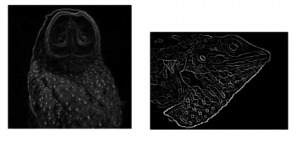
Before reading about the HED, a question that would have popped up is, Why do we want a Deep learning algorithm for such a simple task of edge detection? The answer is that Canny edge detection focuses mainly on local changes and not on the semantics of the image i.e it focuses less on the image’s content. Hence we get less accurate edges.
A technique called Holistically Nested Edge Detection, or HED is a learning-based end-to-end edge detection system that uses a trimmed VGG-like convolutional neural network for an image-to-image prediction task. HED generates the side outputs in the neural network. All the side outputs are fused to make the final output. Let us understand the algorithm in a more detailed manner.
Fig 1.3 Edge Detection using HED
We adopt the VGGNet architecture but make the following modifications:
(a) We connect our side output layer to the last convolutional layer in each stage, respectively conv1 2, conv2 2, conv3 3, conv4 3,conv5 3.
(b) We cut the last stage of VGGNet, including the 5th pooling layer and all the fully connected layers. Also, In-network deconvolutional layers combine the outputs for bi-linear interpolation.
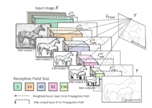
Fig 1.4: HED
The training and testing phase of the HED is covered at the end of the article as its math-heavy section. I would recommend you to have a glance at it to have a better understanding of the model architecture.
Now, let’s talk about the training and testing phase of HED. As I mentioned at the start of the article, this is a math-heavy section so consider this optional learning. I still highly recommend reading through this to grasp the inner workings of HED truly
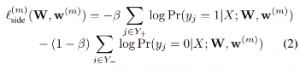
Let us denote the collection of all standard network layer parameters as W, and the network has M side-output layers. Each side-output layer is also associated with a classifier, in which the corresponding weights are denoted as w = (w(1), . . . , w(m)))
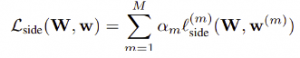
where l<sub>side</sub> denotes the image-level loss function for side outputs. For a typical natural image, the edge/non-edge pixel distribution is heavily biased: 90% of the ground truth is non-edge. A cost-sensitive loss function is with additional trade-off parameters introduced for biased sampling. Specifically, we define the following class-balanced cross-entropy loss function used in the above equation
where ![]()
To directly utilize side-output predictions, we add a “weighted-fusion” layer to the network and (simultaneously) learn the fusion weight during training. Our loss function at the fusion layer Lfuse becomes
![]()
where Dist is the cross-entropy loss. We give the entire objective function as,
![]()
Putting everything together, we minimize the following objective function via standard (back-propagation) stochastic gradient descent:
During testing, given image X, we obtain edge map predictions from both the side output layers and the weighted-fusion layer. The final unified output can be obtained by aggregating these generated edge maps.
Now, we have understood different edge detection algorithms- Traditional and Deep Learning methods. But how do we evaluate the performance of edge detection algorithms or compare different edge detection algorithms?
This brings us to another interesting topic in edge detection – Evaluation Metrics. We will discuss different evaluation metrics for edge detection now.
MSE represents the power of distorting noise that affects the quality of representation.
It is given by
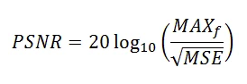
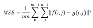 Peak Signal-to-Noise Equation
The peak signal-to-noise ratio (PSNR) is an expression for the ratio between the maximum possible value (power) of a signal and the power of distorting noise that affects the quality of its representation. It is given by
 Structural Similarity Index metric
The Structural Similarity Index metric extracts 3 key features from an image Luminance, Contrast, and Structure. It is given by,
![]()
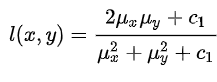
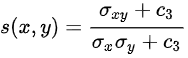
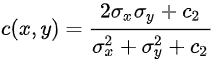
Where,
μx is the average of image X
μy is the average of image Y
σ2x is the variance of X
σ2y is the variance of Y
σxy is the covariance of X and Y
c1 = (k1L)2 and c2 = (k2L)2
k1= 0.01 and k2 = 0.03
L = 2no. of bits per pixel -1
That was a little long article! But we have covered all the concepts of the Canny edge detector and then coded it using OpenCV. We have discussed the 5 steps involved in Canny edge detection, Why the Canny edge detector is better than previous methods. Later we took a glance at the math involved in the HED method. We have also discussed some evaluation metrics to evaluate how well the algorithm performs for the image. Now we can understand the concepts involved in Countour detection, and Hough Line Transforms as they are built above these edge detection algorithms.
The key takeaways of this article are:
Lorem ipsum dolor sit amet, consectetur adipiscing elit,


Thanks for the excellent overview of existing technologies. Check out the recent modification of the classic method - https://kravtsov-development.medium.com/new-high-quality-edge-detector-6757f35a0ee0
Great article with a very good overview of the algorithms.