This article was published as a part of the Data Science Blogathon.
Introduction
K nearest neighbor or KNN is one of the most famous algorithms in classical AI. KNN is a great algorithm to find the nearest neighbors and thus can be used as a classifier or similarity finding algorithm. KNN is great until we are working with a low-dimensional small dataset. A sufficient increase in either dimension or size of the data (total number of rows) renders KNN pretty useless. Increasing the dimension of data points leads to the curse of dimensionality, whereas increasing the number of data points leads to extremely high testing time. In this article, we will not look at the curse of dimensionality. Rather, we will focus on how to use KNN for big datasets.
If we dig a little deeper into the time complexity of KNN, we see that the training time for KNN is O(1) whereas the testing time is O(nd*m) (n=training samples, d=dimension of data, m=test samples). This explodes crazily for big datasets. Let me give you a little more perspective on how it looks regarding numbers. In my testing, a training sample of size (240000 x 728) and a testing sample of size (40000 x 728); the time required to calculate the Euclidean distance for every vector of the test set with every vector in the training set was around 12 hours. I hope this showcase’s the importance of a better strategy to calculate the nearest neighbor. This article discusses a strategy to find the nearest neighbor by approximation distance calculation. Product quantization uses the idea of a lookup table, thus saving us redundant calculations and increasing the speed by many folds.
Calculating Nearest Neighbors Without for/while Loops
The first thing we need to do to identify the top-K nearest neighbors is to make a distance matrix in which each test vector’s distance is calculated with each training vector. Then this matrix can be used to choose the top-K nearest neighbors with the lowest values. We need a distance matrix similar to the one shown in the below diagram. On the first go, it seems that to calculate this, we need to run two loops; one on the training samples and one on testing samples within the training loop.
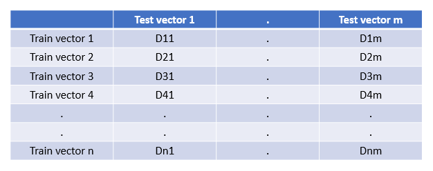
Training Dataset
for test_sample in Test{
for ele in train{
dist[i][j] = dist(ele, test_sample)}
}
But in the subheading, it is mentioned that this can be solved without using any loops. Let’s recall some basic maths to solve this without loops.
Euclidean distance = Sqrt( (a1-a2)² + (b1-b2)² + … + (n1-n2)² )
Note: To fill the above matrix, we can work with square distances because the goal is to find the nearest neighbors, not to calculate the distance on the linear scale.
Let’s use some basic maths to modify the distance equation.
(a-b)² = a² + b² — 2ab
Here’s the interesting part, python can perform multiplication way faster through NumPy rather than using loops. For two random matrices of size (100×100) using the loops, it took 0.47 seconds in my system, whereas direct matrix multiplication took 0.003 seconds only. This means that matrix multiplication is 156 times faster without using loops. The above formula can easily work with matrices as well. Given below is the fastest way to calculate the distance matrix.
def compute_distances_no_loops(self, X):
    dists = -2 * np.dot(X, self.X_train.T) + np.sum(self.X_train**2,    axis=1) + np.sum(X**2, axis=1)[:, np.newaxis]
    return dists1 loops, best of 3: 190 ms per loop
This approach is perfect, but for big datasets, this is impractical due to extremely high memory requirements. Our training sample of size (240000 x 728) and a testing sample of size (40000 x 728) needed 72GB of RAM to calculate the distance matrix.
Calculating Nearest Neighbors with One Loop
We can solve the memory issue by running a loop on each sample of the test vector, thinking of each test vector as one full matrix, and using the above formula to calculate the distances.
def compute_distances_one_loop(self, X):
    dists = np.zeros((num_test, num_train))
    for i in xrange(num_test):
        dists[i, :] = np.sum((self.X_train - X[i, :])**2, axis=1)
    return dists
Product Quantization
Above mentioned techniques might work for fairly large datasets, but when it comes to the actual datasets with billions of rows, it becomes impossible to use these techniques. Here comes the technique of Product quantization for approximate nearest neighbors.
Steps to follow:
- Divide each training vector into chunks of equal size. For our case, we divide each training vector of size (1×600) into (6 times 1×100). Total training vectors are n.
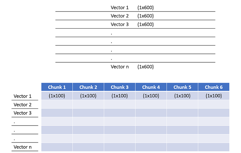
Divide training vectors into chunks of equal size
2. Run a separate K-means algorithm for every chunk. Let’s say for our case K=3. We will 3 centroids get every chunk. Let’s call them (A1, A2, A3), (B1, B2, B3)…, (F1, F2, F3). Note: A1, A2, .., F2, and F3 all are vectors of shape (1×100).
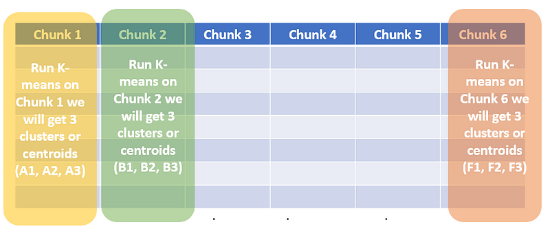
Running K-means of each chunk
3. Assign each block to its closest cluster for each chunk. This is a symbolic representation of the training matrix.
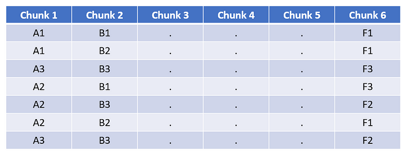
Symbolic representation of training matrix
4. Create a distance map for each chunk. All these blocks will store the distance between two (1×100) sized vectors. For example, if we want to calculate the distance between the centroid A1 and A2, we just use the basic euclidean distance or some other distance like square distance or L1 distance.
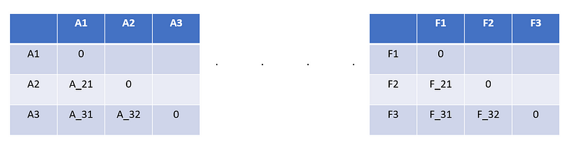
Distance maps of all centroids for each chunk
5. Now we are all set to find the K-nearest neighbors for our test data. Take a sample from test data let’s call it Test[0] and divide it into the same number of chunks.

Divided test sample
6. Assign an ID to each chunk using the smallest euclidean distance between the chunk and all three centroids for the given chunk. Chunk1 will be either assigned to A1, A2, or A3. Chunk2 will be assigned to B1, B2, or B3. The same goes for other chunks.
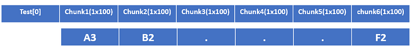
Symbolic representation of a test vector
7. Now compare the Symbolic test vector (Test[0]) with all the training vectors using the distance maps and store their distances.
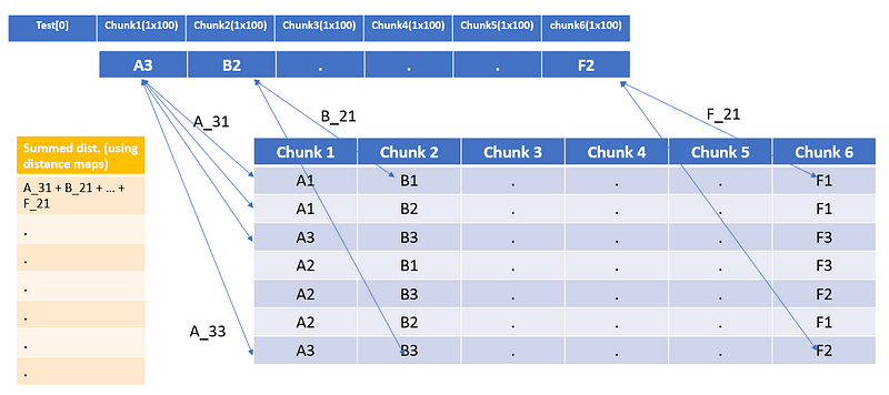
Distance of Test[0] with all training samples
8. Once you have the summed distance, choose the top-k indices that have the lowest summed distance. Nearest neighbors for the given Test[0] vectors will be present at those indices only.
- Test vector(1×600), Train vector (240000×600)
- 6 operations for dividing into chunks.
- Each chunk is compared with 3 centroids (6*3 each operation has 100 elements) and ID is assigned
- Distance calculation using Distance map (6*240000)
Total1 = 6*240000 + 6*3*100 + 6 =1,441,806
Traditional method
- Test vector(1×600), Train vector (240000×600)
- Distance calculation using Distance map (600*240000)
Total2 = 600*240000 = 144,000,000
Conclusion
We can see that the time taken by the traditional K-NN for the above-mentioned case is 100 times more than Product Quantization. Since the testing time for KNN is not linear thus the time difference between the two methods keeps on increasing. The bigger the dataset the slower KNN will perform. One thing to note here is that KNN gives better accuracy than Product quantization, it’s always a fight between accuracy vs speed.
– KNN gives much slower results than product quantization for big datasets.
– Product quantization uses a lookup table to deliver faster results instead of actually calculating distance.
– The speed difference between the two keeps on increasing as the dataset size increases.
– KNN is still more accurate.
– It’s a fight between speed and accuracy.
The media shown in this article is not owned by Analytics Vidhya and is used at the Author’s discretion.


